Deep learning to predict cancer from healthy controls using TCRseq data

Sign up for my newsletter to not miss a post like this

https://divingintogeneticsandgenomics.ck.page/newsletter

The T-cell receptor (TCR) is a special molecule found on the surface of a type of immune cell called a T-cell. Think of T-cells like soldiers in your body’s defense system that help identify and attack foreign invaders like viruses and bacteria.

The TCR is like a sensor or antenna that allows T-cells to recognize specific targets, kind of like how a key fits into a lock. When the TCR encounters a target it recognizes, it sends signals to the T-cell telling it to attack and destroy the invader.

T-cell receptor (TCR) sequencing data is one type of high-throughput sequencing data that provides valuable insights into the immune system’s response to cancer. We can now even get single-cell TCRseq data. In this blog post, we will discuss a deep learning model developed to predict cancer from healthy control using TCRseq data.

This blog post is inspired by the publication De novo prediction of cancer-associated T cell receptors for noninvasive cancer detection. We will use the same training and testing data from https://github.com/s175573/DeepCAT

Download the data.

git clone https://github.com/s175573/DeepCAT

Load in to R:

library(keras)
library(readr)
set.seed(123)
normal_CDR3<- read_tsv("/Users/tommytang/github_repos/DeepCAT/TrainingData/NormalCDR3.txt",
                       col_names = FALSE)

cancer_CDR3<- read_tsv("/Users/tommytang/github_repos/DeepCAT/TrainingData/TumorCDR3.txt",
                       col_names = FALSE)

train_CDR3<- rbind(normal_CDR3, cancer_CDR3)
train_label<- c(rep(0, nrow(normal_CDR3)), rep(1, nrow(cancer_CDR3))) %>% as.numeric()

normal_CDR3_test<- read_tsv("/Users/tommytang/github_repos/DeepCAT/TrainingData/NormalCDR3_test.txt",
                       col_names = FALSE)

cancer_CDR3_test<- read_tsv("/Users/tommytang/github_repos/DeepCAT/TrainingData/TumorCDR3_test.txt",
                       col_names = FALSE)

test_CDR3<- rbind(normal_CDR3_test, cancer_CDR3_test)
test_label<- c(rep(0, nrow(normal_CDR3_test)), rep(1, nrow(cancer_CDR3_test)))

AAindex<- read.table("/Users/tommytang/github_repos/DeepCAT/AAidx_PCA.txt",header = TRUE)

## 20 aa
total_aa<- rownames(AAindex)
total_aa

#>  [1] "A" "R" "N" "D" "C" "E" "Q" "G" "H" "I" "L" "K" "M" "F" "P" "S" "T" "W" "Y"
#> [20] "V"

AAindex is a database of numerical indices representing various physicochemical and biochemical properties of amino acids and pairs of amino acids. In this example, we are not using it. The original paper uses the PCA components as input on top of the CDR3 amino sequences.

Because CDR3s with different lengths usually form distinct loop structures to interact with the antigens, the deepcat paper built five models each for lengths 12 through 16.

one hot encoding for CDR3

encode_one_cdr3<- function(cdr3, length_cutoff){
        res<- matrix(0, nrow = length(total_aa), ncol = length_cutoff)
        cdr3<- unlist(stringr::str_split(cdr3, pattern = ""))
        cdr3<- cdr3[1:length_cutoff]
        row_index<- sapply(cdr3, function(x) which(total_aa==x)[1])
        col_index<- 1: length_cutoff
        res[as.matrix(cbind(row_index, col_index))]<- 1
        return(res)

}
                        
cdr3<- "CASSLKPNTEAFF"

encode_one_cdr3(cdr3, length_cutoff = 12)

#>       [,1] [,2] [,3] [,4] [,5] [,6] [,7] [,8] [,9] [,10] [,11] [,12]
#>  [1,]    0    1    0    0    0    0    0    0    0     0     1     0
#>  [2,]    0    0    0    0    0    0    0    0    0     0     0     0
#>  [3,]    0    0    0    0    0    0    0    1    0     0     0     0
#>  [4,]    0    0    0    0    0    0    0    0    0     0     0     0
#>  [5,]    1    0    0    0    0    0    0    0    0     0     0     0
#>  [6,]    0    0    0    0    0    0    0    0    0     1     0     0
#>  [7,]    0    0    0    0    0    0    0    0    0     0     0     0
#>  [8,]    0    0    0    0    0    0    0    0    0     0     0     0
#>  [9,]    0    0    0    0    0    0    0    0    0     0     0     0
#> [10,]    0    0    0    0    0    0    0    0    0     0     0     0
#> [11,]    0    0    0    0    1    0    0    0    0     0     0     0
#> [12,]    0    0    0    0    0    1    0    0    0     0     0     0
#> [13,]    0    0    0    0    0    0    0    0    0     0     0     0
#> [14,]    0    0    0    0    0    0    0    0    0     0     0     1
#> [15,]    0    0    0    0    0    0    1    0    0     0     0     0
#> [16,]    0    0    1    1    0    0    0    0    0     0     0     0
#> [17,]    0    0    0    0    0    0    0    0    1     0     0     0
#> [18,]    0    0    0    0    0    0    0    0    0     0     0     0
#> [19,]    0    0    0    0    0    0    0    0    0     0     0     0
#> [20,]    0    0    0    0    0    0    0    0    0     0     0     0

This gives you a 20 x 12 matrix, the entry is 1 when the aa is matching the total_aa.

e.g., the first aa is C, so the [5, 1] is 1.

shape the training and testing data

Read my previous post on tensor reshaping.

length_cutoff = 12

train_data<- purrr::map(train_CDR3$X1, ~encode_one_cdr3(.x, length_cutoff = length_cutoff))

# reshape the data to a 2D tensor
train_data<- array_reshape(unlist(train_data), dim = c(length(train_data), 20 * length_cutoff))

# the 20x12 matrix is linearized to a 240 element vector
dim(train_data)

#> [1] 70000   240

test_data<- purrr::map(test_CDR3$X1,  ~encode_one_cdr3(.x, length_cutoff = length_cutoff))
test_data<- array_reshape(unlist(test_data), dim= c(length(test_data), 20* length_cutoff))
dim(test_data)

#> [1] 29851   240

The original paper used a Convolutional Neural Network (CNN), I will use a regular 2 dense-layer model.

y_train <- as.numeric(train_label)
y_test <- as.numeric(test_label)


model <- keras_model_sequential() %>% 
        layer_dense(units = 16, activation = "relu", input_shape = c(20 * length_cutoff)) %>%
        layer_dense(units = 16, activation = "relu") %>%
        layer_dense(units = 1, activation = "sigmoid")


model %>% compile(
        optimizer = "rmsprop",
        loss = "binary_crossentropy",
        metrics = c("accuracy")
)

If one use big epochs, the model will be over-fitted. Set apart 35000 CDR3 sequences for validation.

set.seed(123)
val_indices <- sample(nrow(train_data), 35000)
x_val <- train_data[val_indices,]
partial_x_train <- train_data[-val_indices,]

y_val <- y_train[val_indices]
partial_y_train <- y_train[-val_indices]

history <- model %>% fit(partial_x_train, 
                         partial_y_train, 
                         epochs = 20, 
                         batch_size = 512, 
                         validation_data = list(x_val, y_val)
)

plot(history)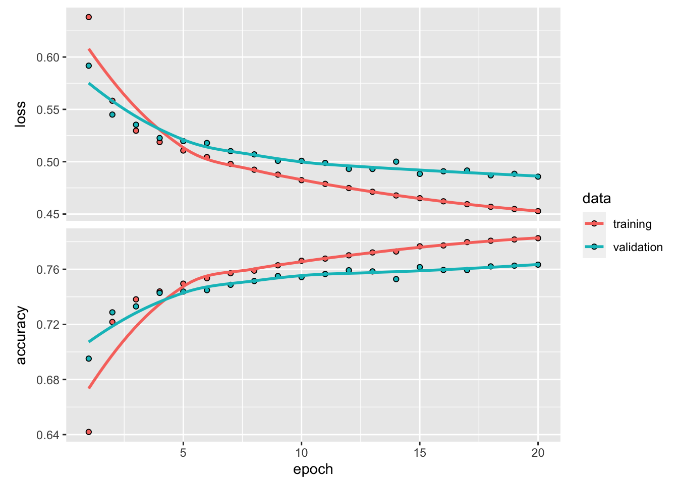

final training and testing

model %>% fit(train_data, y_train, epochs = 20, batch_size = 512)
results <- model %>% evaluate(test_data, y_test)
results

#>      loss  accuracy 
#> 0.4229931 0.8065391

~80% accuracy. Not bad…

Let’s increase the number of units in each layer.

model <- keras_model_sequential() %>% 
        layer_dense(units = 64, activation = "relu", input_shape = c(20 * length_cutoff)) %>%
        layer_dense(units = 64, activation = "relu") %>%
        layer_dense(units = 1, activation = "sigmoid")


model %>% compile(
        optimizer = "rmsprop",
        loss = "binary_crossentropy",
        metrics = c("accuracy")
)

val_indices <- sample(nrow(train_data), 35000)
x_val <- train_data[val_indices,]
partial_x_train <- train_data[-val_indices,]

y_val <- y_train[val_indices]
partial_y_train <- y_train[-val_indices]

history <- model %>% fit(partial_x_train, 
                         partial_y_train, 
                         epochs = 20, 
                         batch_size = 512, 
                         validation_data = list(x_val, y_val)
)

plot(history)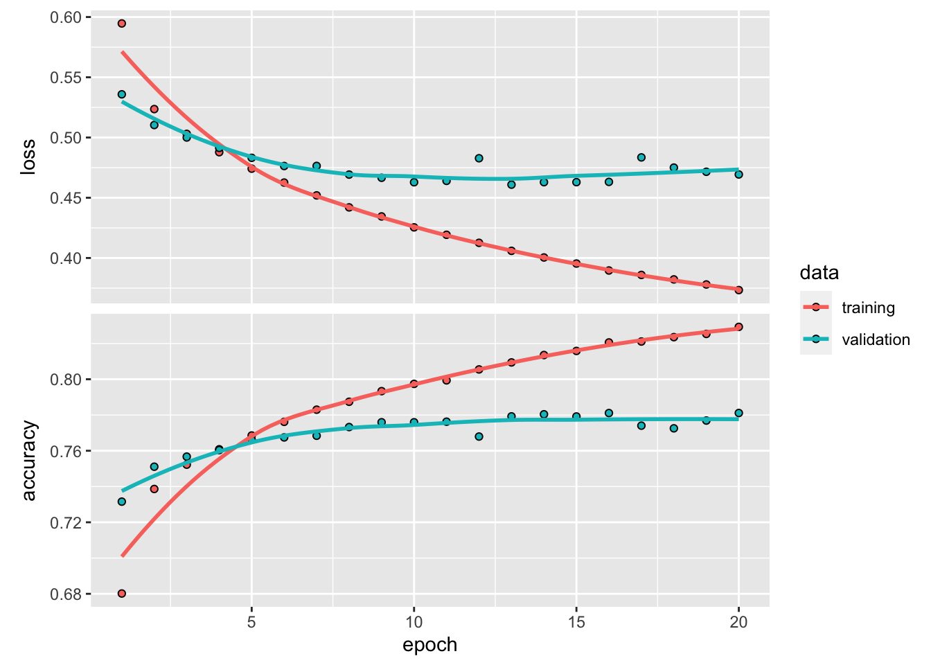

with more units (neurons) in each layer, overfitting occurs much faster. after 10 epoch, the validation accuracy starts to plateau.

model %>% fit(train_data, y_train, epochs = 10, batch_size = 512)
results <- model %>% evaluate(test_data, y_test)
results

#>      loss  accuracy 
#> 0.3731814 0.8282135

predict(model, test_data[1:10, ])

#>             [,1]
#>  [1,] 0.08662453
#>  [2,] 0.23022524
#>  [3,] 0.21670932
#>  [4,] 0.03327328
#>  [5,] 0.03596783
#>  [6,] 0.07136077
#>  [7,] 0.06769678
#>  [8,] 0.03962836
#>  [9,] 0.16300359
#> [10,] 0.36324140

How to improve the accuracy by using biology domian knowledge?

It is surprising to me that using only the CDR3 aa sequences can reach an accuracy of 80%. How can we further improve it?

• we can add the AA properties
• add the VDJ usage
• add HLA typing for each sample

Further reading

• DeepTCR is a deep learning framework for revealing sequence concepts within T-cell repertoires

• Deep learning reveals predictive sequence concepts within immune repertoires to immunotherapy