Introduction
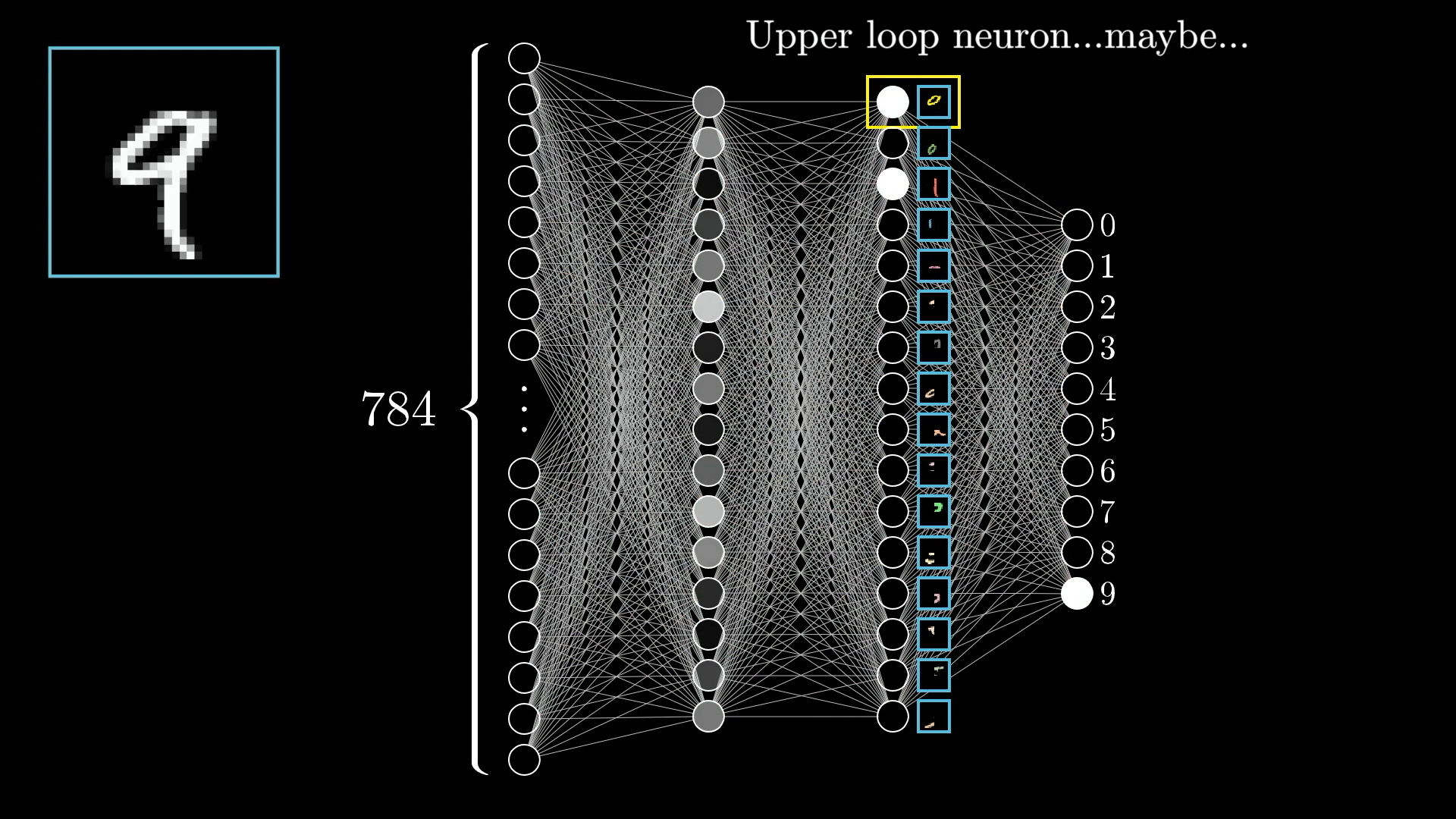
Are you a machine learning practitioner or data analyst looking to broaden your skill set? Look nowhere else! This blog post will offer an introduction to deep learning, which is currently the hottest topic in machine learning. Using the well-known MNIST dataset) and the Keras package, we will investigate the potential of deep learning.
A high-level deep learning package called Keras, which is based on TensorFlow, enables quick and simple experimentation with deep neural networks. Anyone can run a deep learning model in a matter of hours with Keras. No prior knowledge is necessary as I walk you through the fundamentals of Keras, from installation to creating a deep learning model from scratch!
I recommend watching the youtube series from 3blue1brown: https://www.3blue1brown.com/topics/neural-networks to get intuitive understanding of how neural network works.
Josh Starmer also has very nice videos on this topic https://statquest.org/video-index/.
Install the package
#install.packages("keras") install the keras R package
library(keras)
#install_keras(version = "release")  install the core Keras library and TensorFlow
set.seed(123)
It installs tensorflow to /Users/tommytang/Library/r-miniconda/envs/r-reticulate/bin/python
To set the value of RETICULATE_PYTHON, insert Sys.setenv(RETICULATE_PYTHON = PATH) into your project’s .Rprofile, where PATH is your preferred Python binary.
I added this
Sys.setenv(RETICULATE_PYTHON = "/Users/tommytang/Library/r-miniconda/envs/r-reticulate/bin/python") to my .Rprofile in the same folder as the .Rproj.
Take a read https://rstudio.github.io/reticulate/articles/versions.html to further understand how to configure python path inside Rstudio.
Get the data and do exploratory data analysis
library(reticulate)
use_condaenv("r-reticulate")
mnist<- dataset_mnist()
split the training and testing sets
train_images<- mnist$train$x
train_labels<- mnist$train$y
train_labels<- to_categorical(train_labels)

test_images<- mnist$test$x
test_labels<- mnist$test$y
test_labels<- to_categorical(test_labels)
The training sets is a 3D tensor. Tensors are just a fancy way to say multi-dimentional array. A 2D tensor is just a matrix.
dim(train_images)#> [1] 60000 28 28It is an array of 60,000 matrices of 28x28 integers. Each matrix is a grayscale image:
# get the fifth matrix
digit<- train_images[5, ,]
dim(digit)
#> [1] 28 28plot(as.raster(digit, max = 255))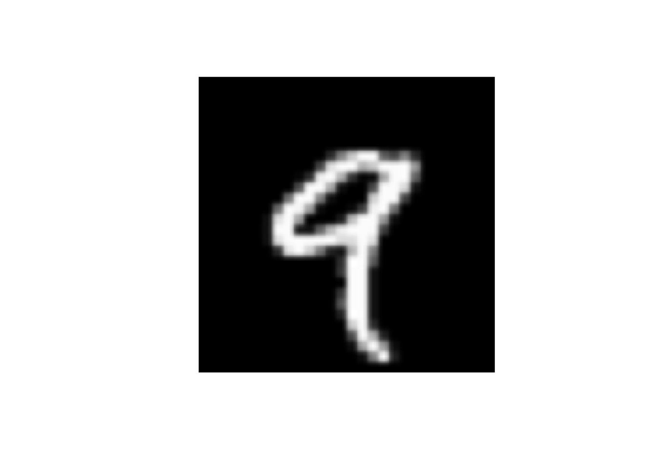
It is a matrix denoting the image of 9.
reshape the data into 2D tensor
train_images<- array_reshape(train_images, c(60000, 28 * 28))
train_images<- train_images/255


test_images<- array_reshape(test_images, c(10000, 28 * 28))
test_images<- test_images/255dim(train_images)#> [1] 60000 784Now, it becomes a 6000 x 784 2D tensor.
exploratory data analysis
Before doing any analysis, exploratory data analysis (EDA) is the first thing you should do.
Let’s use irlba (Fast Truncated Singular Value Decomposition and Principal Components Analysis for Large Dense and Sparse Matrices) for PCA. irlba is both faster and more memory efficient than the usual R svd function for computing a few of the largest singular vectors and corresponding singular values of a matrix.
Read my old post on PCA if you want to learn more.
library(irlba)
library(ggplot2)
library(dplyr)

dim(train_images)
#> [1] 60000 784pca.results <- irlba(A = train_images, nv = 30)
image_pc_loadings<- pca.results$u
colnames(image_pc_loadings)<- paste0("PC_", 1:30)
labels_vector<- apply(mnist$train$y, 1, max) %>%
as.character()
image_pc_df<- image_pc_loadings %>%
as.data.frame() %>%
dplyr::bind_cols(label = labels_vector)
ggplot(image_pc_df, aes(x=PC_1, y = PC_2)) +
scattermore::geom_scattermore(aes(color = label)) +
theme_classic(base_size = 14)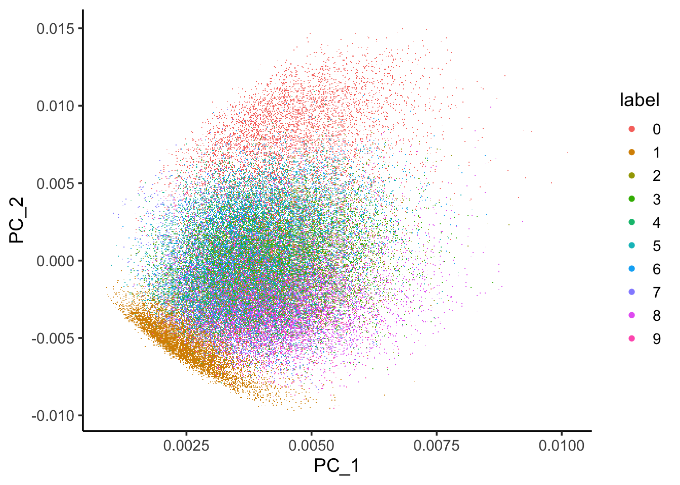
You can see some structure of the data by using PCA.
Let’s use uwot for UMAP dimension reduction which may give you a better visualization of
the data structure.
UMAP is a form of non-linear dimension reduction technique that is useful for visualizing the data. It is very popular in single-cell data analysis.
library(uwot)
mnist_umap <- umap(train_images, n_neighbors = 15, min_dist = 0.001, verbose = TRUE, pca = 50)

colnames(mnist_umap)<- c("UMAP_1", "UMAP_2")
mnist_umap<- bind_cols(mnist_umap, label = labels_vector)

ggplot(mnist_umap, aes(x=UMAP_1, y = UMAP_2)) +
        scattermore::geom_scattermore(aes(color = label)) +
        theme_classic(base_size = 14)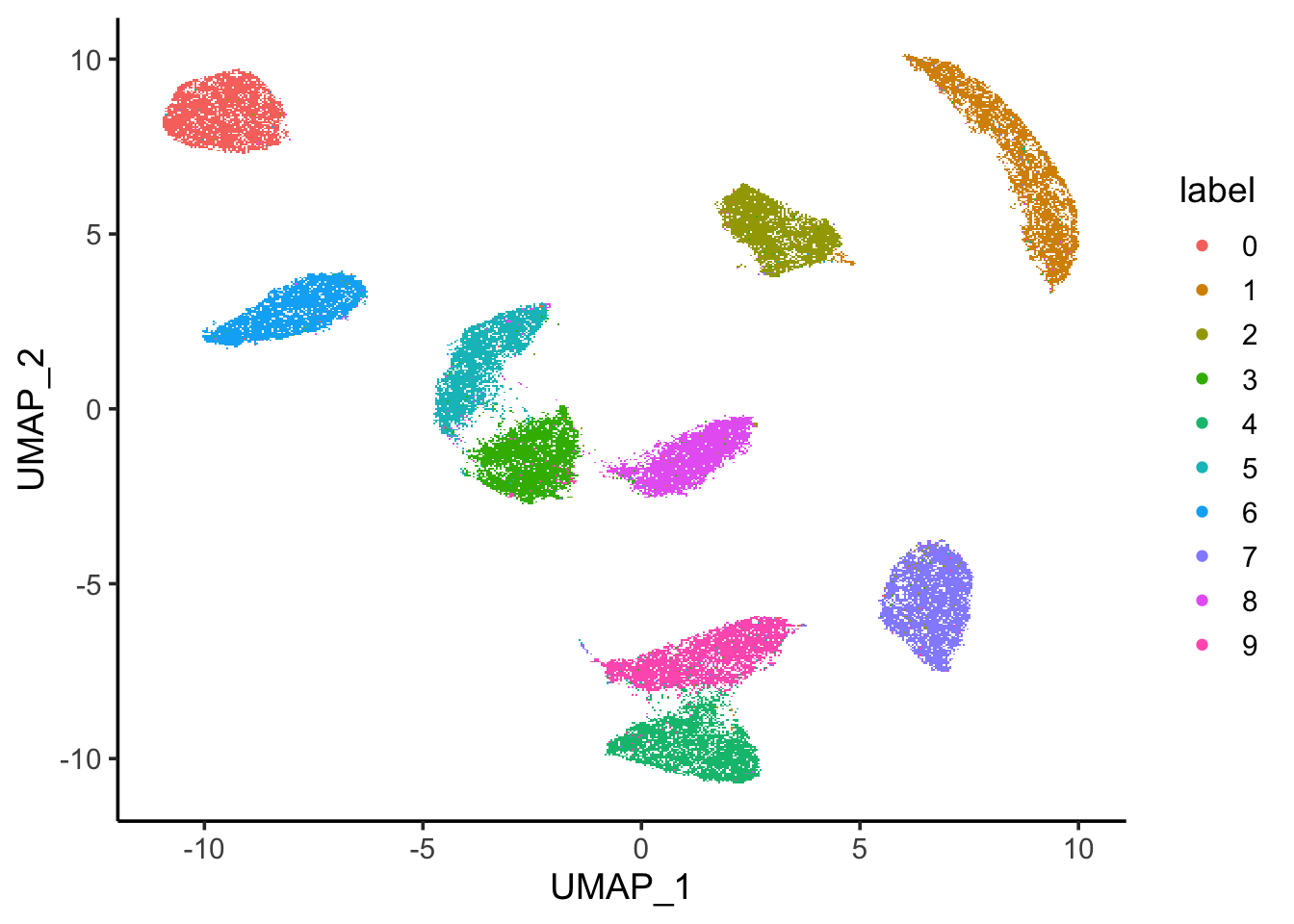
Wow. most of the images are separated by its digits. Note that when you have many data points, they plot on top of each other. The best way is to calculate a metric on the cluster purity rather than judge by your eyes.
I think most people using UMAPs don't realize that when points are colored in order (the default way of plotting), buried colors make the points appear to be (much!) better grouped together than they really are.
— Lior Pachter (@lpachter) March 10, 2023
This figure is from the supplement of https://t.co/a0Ltb5lCGN pic.twitter.com/ZMVYB9bJTW
See also my previous blog post How to deal with overplotting without being fooled.
Train the network
Now, let’s construct the network using two dense layers.
network<- keras_model_sequential() %>%
        layer_dense(unit= 512, activation = "relu", input_shape = c(28 * 28))%>%
        layer_dense(units = 10, activation = "softmax")
The last layer has 10 neurons because we are predicting the images to be 0-9 and the activation function is softmax
to give a probability of the image predicted to 0-9. The sum of them will be 1.
In the compilation step, you may configure the learning process by specifying the optimizer and loss function(s) the model should employ as well as the metrics you wish to track while it is being trained.
Compile the network by telling the loss function and metrics. categorical_crossentropy is good for categorical classifications.
For binary classification, you will use binary_crossentropy.
network %>%
        compile(optimizer = "rmsprop",
                loss = "categorical_crossentropy",
                metrics= c("accuracy"))
compile() function modifies the network in place (rather than returning a new network object, as is more conventional in R.
Finally, the training:
network %>%
        fit(train_images, train_labels, epochs = 5, batch_size = 128)
The network will iterate on the training data in mini-batches of 128 samples, 5 times over(each iteration over all the training data is called an epoch).
evaluate the model
metrics<- network %>% evaluate(test_images, test_labels)
metrics
#> loss accuracy
#> 0.08828809 0.9746000298% accuracy! impressive.
How does random forest perform?
Random forest is my go-to for machine learning after linear regression, before deep learning.
Let’s see how it performs using tidymodels.
A book for you to read https://www.tidymodels.org/books/tmwr/.
library(tidymodels)
set.seed(123)

data_train<- train_images
colnames(data_train)<- paste0("feature", 1:784)
data_train<- bind_cols(as.data.frame(data_train), label =  apply(mnist$train$y, 1, max) %>%
        as.character())

data_test<- test_images
colnames(data_test)<- paste0("feature", 1:784)
data_test<- bind_cols(as.data.frame(data_test), label = apply(mnist$test$y, 1, max) %>%
        as.character())

# it is key to turn it to a factor for classification
data_train$label<- factor(data_train$label)
data_test$label<- factor(data_test$label)
It turns out 60,000 images is a lot for random forest and it takes hours to fit the model. what impresses me about the deep learning model apart from its accuracy is its speed. For 60,000 images, it finished in seconds.
Let me just randomly take 3000 images.
data_train<- dplyr::sample_n(data_train, size = 3000)
dim(data_train)
#> [1] 3000 785library(tidymodels)
library(tictoc)
tic()
rf_recipe <-
recipe(formula = label ~ ., data = data_train)
## feature importance sore to TRUE, one can tune the trees and mtry
rf_spec <- rand_forest() %>%
set_engine("randomForest", importance = TRUE) %>%
set_mode("classification")
rf_workflow <- workflow() %>%
add_recipe(rf_recipe) %>%
add_model(rf_spec)
rf_fit <- fit(rf_workflow, data = data_train)
res<- predict(rf_fit, new_data = data_test) %>%
bind_cols(data_test %>% select(label))
toc()#> 193.75 sec elapsedaccuracy(res, truth = label, estimate = .pred_class)#> # A tibble: 1 × 3
#> .metric .estimator .estimate
#> <chr> <chr> <dbl>
#> 1 accuracy multiclass 0.936## confusion matrix,
res %>% conf_mat(truth = label, estimate = .pred_class)#> Truth
#> Prediction 0 1 2 3 4 5 6 7 8 9
#> 0 967 0 11 4 1 10 17 2 4 6
#> 1 1 1121 4 3 1 8 4 15 6 7
#> 2 1 2 958 15 4 2 3 27 4 3
#> 3 0 3 6 930 0 37 1 4 23 12
#> 4 0 0 11 1 931 6 11 6 9 27
#> 5 5 2 1 21 0 793 9 0 15 8
#> 6 3 3 10 2 7 13 910 0 6 3
#> 7 1 0 19 12 0 2 0 936 5 6
#> 8 2 4 9 17 2 14 3 6 883 8
#> 9 0 0 3 5 36 7 0 32 19 929An accuracy of this un-tuned random forest model gives 93.6% accuracy. Not bad! However, it is very slow.
Calling P the number of simultaneous workers you have) the complexities should be (depending on the implementations) :
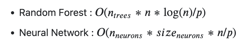
you should expect random forests to be slower than neural networks
Take home messages
Running a deep learning model with Keras is not hard (with less than 20 lines of code). What is harder? 👇
Defining the right question. This is always the most challenging part. How can deep learning help with this certain problem? have you tried conventional ML methods? Do you have the right/size data? When you have millions of data points, the accuracy of deep learning models can be really high.
Getting the data into the proper format and reshaping the tensor into the right dimension is hard. In the next post, I will walk you through how to manipulate and do calculations for the arrays (tensors).
Tuning the model is hard. What are some hyper-parameters to try? We have not tuned the hyperparameter in this example. In a future post. I will show you how to tune the epoch hyper-parameter to avoid over-fitting.
Making sense of the model is hard (DL is notorious for its black box). what can you learn from the model. Random forest gives you the feature importance, so you can study the features. Deep learning is like a black box. It performs well, but you do not really know what’s going on within the black box.
How can you improve it by adding additional information to the input (domain knowledge is the key)? In a future post, I will show you how to use T cell receptor (TCR) sequence to predict cancer and what information we can add to the input to improve the accuracy of prediction.