In my last blog post, I showed that pearson gene correlation for single-cell data has flaws because of the sparsity of the count matrix.
One way to get around it is to use the so called meta-cell. One can use KNN to find the K nearest neighbors and collapse them into a meta-cell. You can implement it from scratch, but one should not re-invent the wheel. For example, you can use metacells.
I want to keep the workflow within R and I found hdWGCNA has a function to do that. What’s even better, it can be directly used with Seurat.
For gene co-expression network analysis, you must have heard of WGCNA, it has been cited over 13,500 times. WGCNA is designed for bulk-RNAseq. For single-cell, hdWGCNA creates metacell using KNN and then use the same WGCNA workflow.
Let’s use the same pbmc data to try this tool.
Load libraries
library(dplyr)
library(Seurat)
library(patchwork)
library(ggplot2)
library(ComplexHeatmap)
library(SeuratData)
library(hdWGCNA)
library(WGCNA)
set.seed(1234)
prepare the data
data("pbmc3k")

pbmc3k
#> An object of class Seurat
#> 13714 features across 2700 samples within 1 assay
#> Active assay: RNA (13714 features, 0 variable features)## routine processing
pbmc3k<- pbmc3k %>%
NormalizeData(normalization.method = "LogNormalize", scale.factor = 10000) %>%
FindVariableFeatures(selection.method = "vst", nfeatures = 2000) %>%
ScaleData() %>%
RunPCA(verbose = FALSE) %>%
FindNeighbors(dims = 1:10, verbose = FALSE) %>%
FindClusters(resolution = 0.5, verbose = FALSE) %>%
RunUMAP(dims = 1:10, verbose = FALSE)
Idents(pbmc3k)<- pbmc3k$seurat_annotations
pbmc3k<- pbmc3k[, !is.na(pbmc3k$seurat_annotations)]some functions we will use
matrix_to_expression_df<- function(x, obj){
        df<- x %>%
                as.matrix() %>%
                as.data.frame() %>%
                tibble::rownames_to_column(var= "gene") %>%
                tidyr::pivot_longer(cols = -1, names_to = "cell", values_to = "expression") %>%
                tidyr::pivot_wider(names_from = "gene", values_from = expression) %>%
                left_join(obj@meta.data %>%
                                  tibble::rownames_to_column(var = "cell"))
        return(df)
}


get_expression_data<- function(obj, assay = "RNA", slot = "data",
                               genes = NULL, cells = NULL){
        if (is.null(genes) & !is.null(cells)){
                df<- GetAssayData(obj, assay = assay, slot = slot)[, cells, drop = FALSE] %>%
                        matrix_to_expression_df(obj = obj)
        } else if (!is.null(genes) & is.null(cells)){
                df <- GetAssayData(obj, assay = assay, slot = slot)[genes, , drop = FALSE] %>%
                        matrix_to_expression_df(obj = obj)
        } else if (is.null(genes & is.null(cells))){
                df <- GetAssayData(obj, assay = assay, slot = slot)[, , drop = FALSE] %>%
                        matrix_to_expression_df(obj = obj)
        } else {
                df<- GetAssayData(obj, assay = assay, slot = slot)[genes, cells, drop = FALSE] %>%
                        matrix_to_expression_df(obj = obj)
        }
        return(df)
}
construct metacell
pbmc3k <- SetupForWGCNA(
  pbmc3k,
  gene_select = "fraction", # the gene selection approach
  fraction = 0.05, # fraction of cells that a gene needs to be expressed in order to be included
  wgcna_name = "tutorial" # the name of the hdWGCNA experiment
)


# construct metacells in each group.
# choosing K is an art.
pbmc3k <- MetacellsByGroups(
  seurat_obj = pbmc3k,
  group.by = c("seurat_annotations", "orig.ident"), # specify the columns in seurat_obj@meta.data to group by
  k = 10, # nearest-neighbors parameter
  max_shared = 5, # maximum number of shared cells between two metacells
  ident.group = 'seurat_annotations' # set the Idents of the metacell seurat object
)
routine processing for the meta-cell seurat object
# extract the metacell seurat object
pbmc_metacell <- GetMetacellObject(pbmc3k)

pbmc_metacell <- pbmc_metacell %>%
        NormalizeData(normalization.method = "LogNormalize", scale.factor = 10000) %>%
        FindVariableFeatures(selection.method = "vst", nfeatures = 2000) %>%
        ScaleData() %>%
        RunPCA(verbose = FALSE) %>%
        FindNeighbors(dims = 1:10, verbose = FALSE) %>%
        FindClusters(resolution = 0.5, verbose = FALSE) %>%
        RunUMAP(dims = 1:10, verbose = FALSE)

Idents(pbmc_metacell)<- pbmc_metacell$seurat_annotations

p1<- DimPlot(pbmc3k, reduction = "umap", label = TRUE, repel = TRUE) +
        NoLegend() + ggtitle("single cell")

p2<- DimPlot(pbmc_metacell, reduction = "umap", label = TRUE, repel = TRUE) +
        NoLegend() + ggtitle("meta cell")

p1 + p2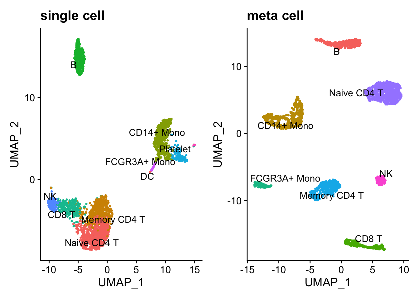
Note, DCs and Platelet are dropped in the metacell because the number of cells are too few. Overall, the metacell clustering makes sense. Interestingly, Memory CD4 T and Naive CD4 T cells are more distinct after constructing metacells.
co-expression network analysis
Let’s focus on naive NK cells
Next we will select the “soft power threshold”. This is an extremely important step in the hdWGNCA pipleine (and for vanilla WGCNA). hdWGCNA constructs a gene-gene correlation adjacency matrix to infer co-expression relationships between genes. The correlations are raised to a power to reduce the amount of noise present in the correlation matrix, thereby retaining the strong connections and removing the weak connections. Therefore, it is critical to determine a proper value for the soft power threshold.
pbmc3k<- SetDatExpr(
  pbmc3k,
  group_name = "NK", # the name of the group of interest in the group.by column
  group.by='seurat_annotations',
  assay = 'RNA', # using RNA assay
  slot = 'data', # using normalized data
  use_metacells=TRUE
)
#> ..Excluding 28 genes from the calculation due to too many missing samples or zero variance.# Test different soft powers:
# https://stackoverflow.com/questions/57467678/wgcna-sharing-namespaces-for-statistical-methods
bicor = WGCNA::bicor
pbmc3k <- TestSoftPowers(
pbmc3k,
networkType = 'signed' # you can also use "unsigned" or "signed hybrid"
)#> pickSoftThreshold: will use block size 3829.
#> pickSoftThreshold: calculating connectivity for given powers...
#> ..working on genes 1 through 3829 of 3829
#> Power SFT.R.sq slope truncated.R.sq mean.k. median.k. max.k.
#> 1 1 0.10400 10.700 0.979 1.97e+03 1.97e+03 2140.00
#> 2 2 0.00146 0.588 0.972 1.03e+03 1.03e+03 1220.00
#> 3 3 0.01420 -1.240 0.976 5.53e+02 5.51e+02 714.00
#> 4 4 0.09060 -2.310 0.982 3.02e+02 3.00e+02 426.00
#> 5 5 0.21600 -2.910 0.989 1.68e+02 1.67e+02 259.00
#> 6 6 0.33800 -3.080 0.985 9.56e+01 9.40e+01 160.00
#> 7 7 0.49900 -3.590 0.977 5.54e+01 5.41e+01 105.00
#> 8 8 0.62700 -3.990 0.968 3.27e+01 3.16e+01 70.60
#> 9 9 0.72000 -4.090 0.953 1.96e+01 1.88e+01 49.30
#> 10 10 0.77700 -4.090 0.922 1.20e+01 1.14e+01 35.60
#> 11 12 0.88400 -3.970 0.921 4.70e+00 4.35e+00 20.40
#> 12 14 0.94900 -3.680 0.941 1.97e+00 1.76e+00 13.30
#> 13 16 0.50900 -4.680 0.408 8.87e-01 7.47e-01 9.55
#> 14 18 0.50200 -4.040 0.400 4.27e-01 3.32e-01 7.44
#> 15 20 0.48900 -3.490 0.399 2.21e-01 1.54e-01 6.13
#> 16 22 0.44500 -3.760 0.374 1.23e-01 7.36e-02 5.25
#> 17 24 0.42900 -3.310 0.370 7.45e-02 3.62e-02 4.61
#> 18 26 0.41700 -3.000 0.376 4.88e-02 1.82e-02 4.13
#> 19 28 0.40500 -3.140 0.355 3.44e-02 9.39e-03 3.75
#> 20 30 0.39700 -2.930 0.360 2.59e-02 4.92e-03 3.43# plot the results:
plot_list <- PlotSoftPowers(pbmc3k)#> Power SFT.R.sq slope truncated.R.sq mean.k. median.k. max.k.
#> 1 1 0.104482638 10.6974118 0.9794689 1966.24968 1967.49111 2136.0980
#> 2 2 0.001455736 0.5883556 0.9719670 1031.60352 1031.10783 1221.3620
#> 3 3 0.014219159 -1.2409468 0.9755679 552.54983 550.97194 713.9150
#> 4 4 0.090647219 -2.3128225 0.9822797 301.99242 300.13466 425.8164
#> 5 5 0.216410422 -2.9075671 0.9886817 168.33374 166.55123 258.7715
#> 6 6 0.337671091 -3.0818337 0.9849525 95.64999 93.97877 160.0256# assemble with patchwork
wrap_plots(plot_list, ncol=2)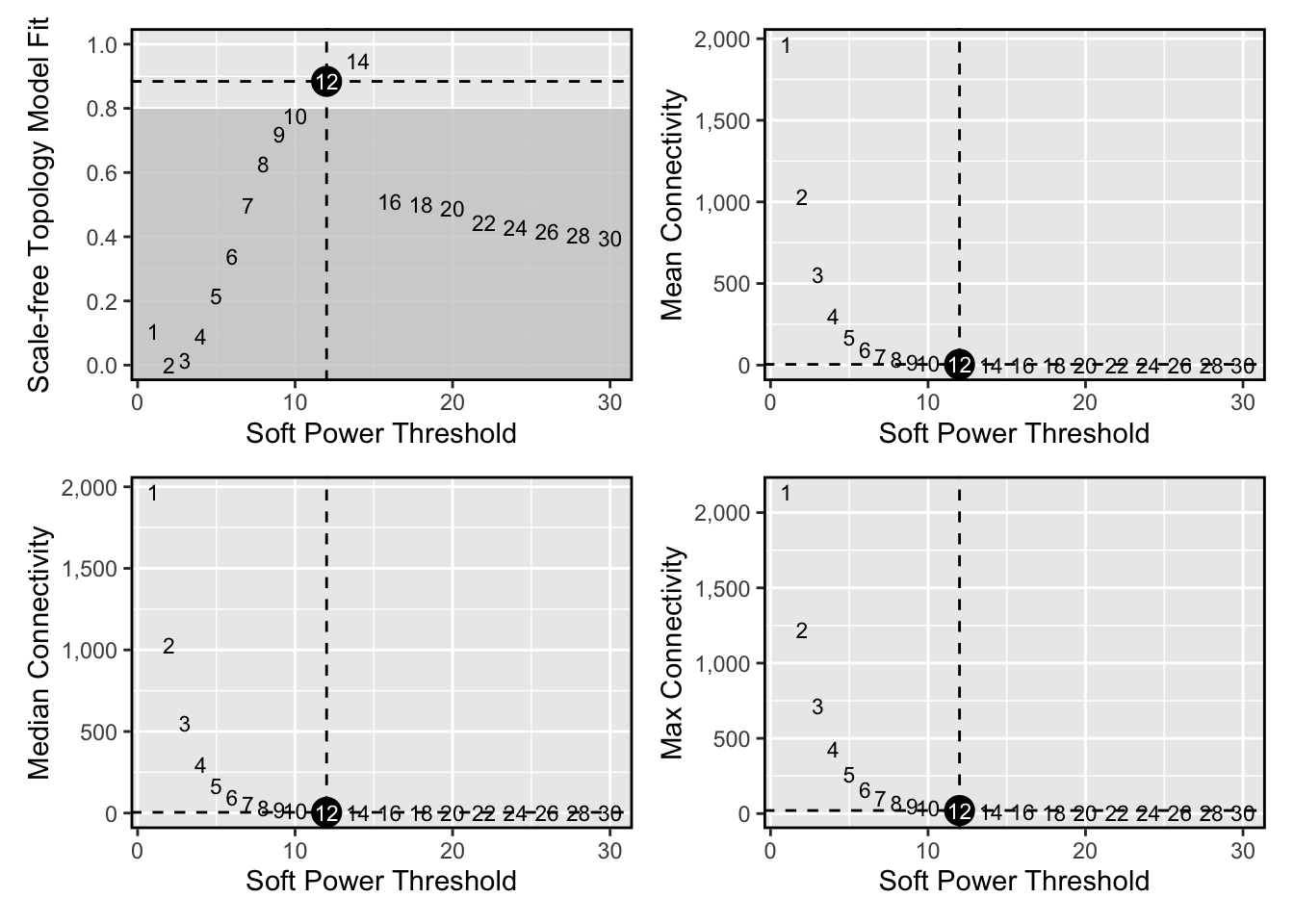
we select soft_power=12 based on the plot above.
# construct co-expression network:
pbmc3k <- ConstructNetwork(
  pbmc3k, soft_power=12,
  setDatExpr=FALSE,
  tom_name = 'NK', # name of the topoligical overlap matrix written to disk
  overwrite_tom = TRUE
)
#> Calculating consensus modules and module eigengenes block-wise from all genes
#> Calculating topological overlaps block-wise from all genes
#> Flagging genes and samples with too many missing values...
#> ..step 1
#> TOM calculation: adjacency..
#> ..will not use multithreading.
#> Fraction of slow calculations: 0.000000
#> ..connectivity..
#> ..matrix multiplication (system BLAS)..
#> ..normalization..
#> ..done.
#> ..Working on block 1 .
#> ..Working on block 1 .
#> ..merging consensus modules that are too close..PlotDendrogram(pbmc3k, main='NK hdWGCNA Dendrogram')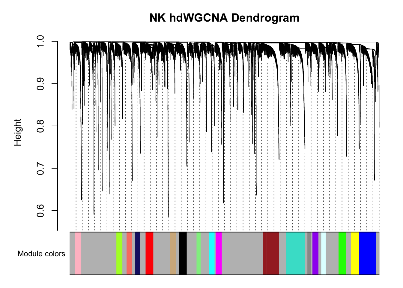
There are multiple co-expression modules are recovered. Ignore the grey module.
# get the module assignment table:
modules <- GetModules(pbmc3k)

head(modules)
#> gene_name module color
#> NOC2L NOC2L blue blue
#> HES4 HES4 grey grey
#> ISG15 ISG15 grey grey
#> TNFRSF4 TNFRSF4 magenta magenta
#> SDF4 SDF4 lightgreen lightgreen
#> UBE2J2 UBE2J2 grey greytable(modules$module)#>
#> blue grey magenta lightgreen brown green
#> 208 2078 75 50 197 96
#> salmon black grey60 midnightblue turquoise yellow
#> 68 95 54 61 229 102
#> greenyellow tan pink red purple lightcyan
#> 74 72 80 96 74 55
#> cyan
#> 65modules %>% filter(gene_name == "PRF1")#> gene_name module color
#> PRF1 PRF1 turquoise turquoisemodules %>% filter(gene_name == "GZMM")#> gene_name module color
#> GZMM GZMM turquoise turquoise# GZMB is not in the same module...
modules %>% filter(gene_name == "GZMB")#> gene_name module color
#> GZMB GZMB grey greyI cherry picked PRF1 and GZMM.
correlation for metacell
Let’s see how it looks for single cell first:
genes<- c("PRF1", "GZMM")

expression_data<- get_expression_data(pbmc3k, genes = genes)

# https://github.com/LKremer/ggpointdensity
# ggpubr to add the correlation

ggplot(expression_data, aes(x= PRF1, y = GZMM)) +
        #geom_smooth(method="lm") +
        geom_point(size = 0.8) +
        facet_wrap(~seurat_annotations) +
        ggpubr::stat_cor(method = "pearson")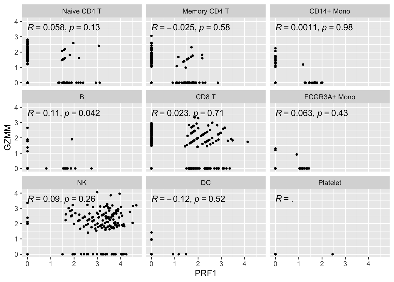
For metacell
ggplot(get_expression_data(pbmc_metacell, genes = genes), aes(x= PRF1, y = GZMM)) +
        geom_smooth(method="lm") +
        geom_point(size = 0.8) +
        facet_wrap(~seurat_annotations) +
        ggpubr::stat_cor(method = "pearson")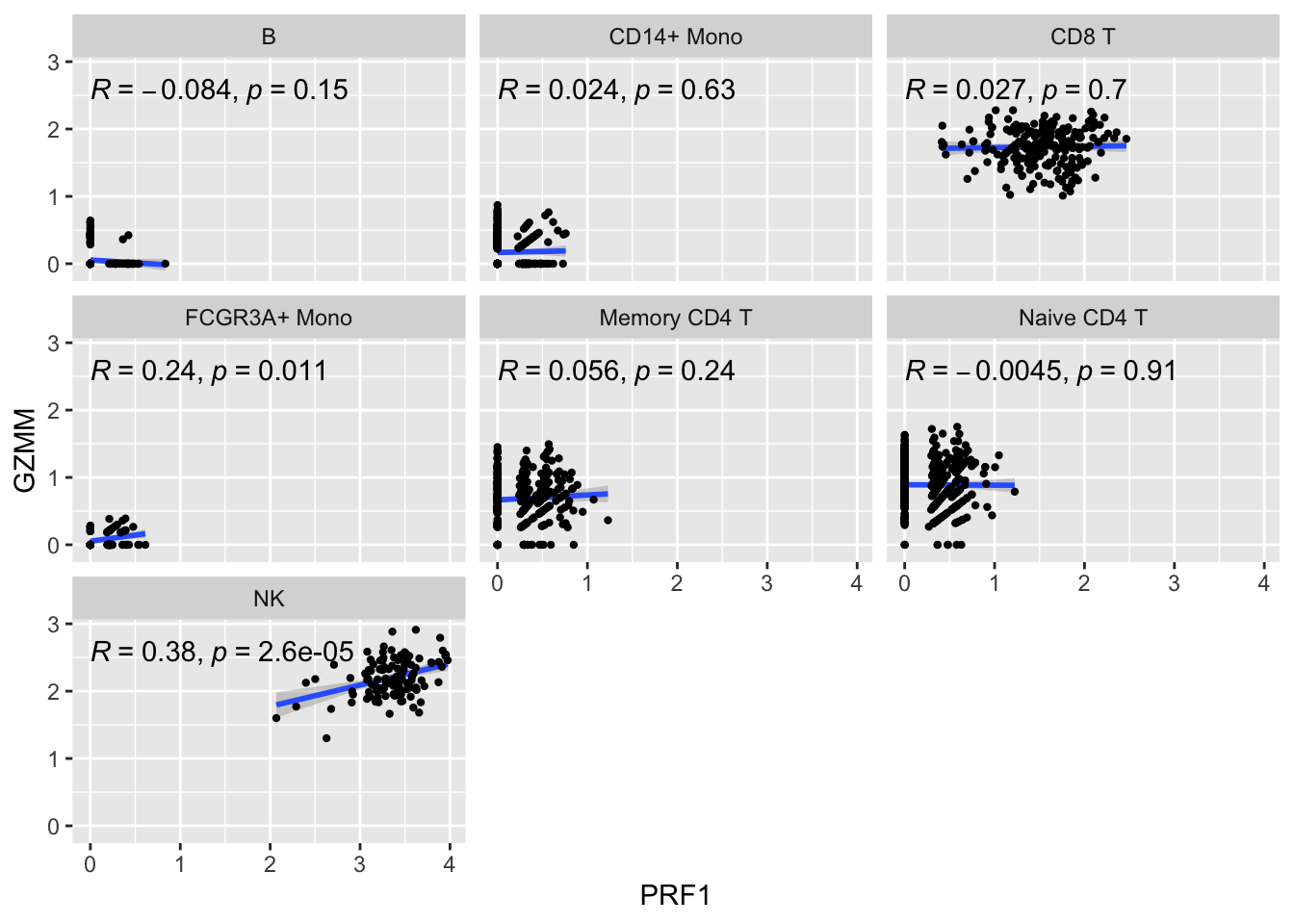
The metacell correlation scatter plot looks better than the single-cell one.
Take home messages:
Using metacell may help with single-cell RNA-seq gene correlation/co-expression analysis.
Do not re-invent the wheel. Use existing tools but do not trust them blindly.
Choosing the right K in the KNN is an art. Like many other bioinformatics problems, choosing the right parameters and cutoffs can be a major task itself!
Always visualize the data (EDA). Is the correlation looks convincing to you in the scatter plot?
When you have large N, the p-value will be tiny. Focus on the effect size (the correlation coefficient in this case).