clustering scATACseq data: the TF-IDF way

May 3, 2019 15 min read R, single-cell, scATACseq, bioinformatics

scATACseq data are very sparse. It is sparser than scRNAseq. To do clustering of scATACseq data, there are some preprocessing steps need to be done.

I want to reproduce what has been done after reading the method section of these two recent scATACseq paper:

A Single-Cell Atlas of In Vivo Mammalian Chromatin Accessibility Darren et.al Cell 2018

Latent Semantic Indexing Cluster Analysis

In order to get an initial sense of the relationship between individual cells, we first broke the genome into 5kb windows and then scored each cell for any insertions in these windows, generating a large, sparse, binary matrix of 5kb windows by cells for each tissue. Based on this matrix, we retained the top 20,000 most commonly used sites in each tissue (this number could extend a little above 20,000 because we included tied sites at the threshold) and then filtered out the bottom 5% of cells in terms of the number of 5kb windows with any insertions. We then reduced the dimensionality of these large binary matrices using a term frequency-inverse document frequency (‘‘TF-IDF’’) transformation. To do this, we first weighted all the sites for individual cells by the total number of sites accessible in that cell (‘‘term frequency’’). We then multiplied these weighted values by log(1 + the inverse frequency of each site across all cells), the ‘‘inverse document frequency.’’ We then used singular value decomposition on the TF-IDF matrix to generate a lower dimensional representation of the data by only retaining the 2nd through 10th dimensions (because the first dimension tends to be highly correlated with read depth). These LSI-transformed scores of accessibility were then standardized by row (i.e., mean subtracted and divided by standard deviation), capped at ± 1.5, and used to bi-cluster cells and windows based on cosine distances using the ward algorithm in R. Visual examination of the resulting heatmaps identified between 2 and 7 distinct clusters of cells, de- pending on the tissue. These relatively crude groups of cells were used for peak calling (described below) to maintain enough cells in each group for identifying peaks while also retaining sufficient sensitivity to identify peaks that were restricted to subset of cells.

t-distributed Stochastic Neighbor Embedding and Iterative Cluster Analysis

To take a more holistic approach to understanding the relationships of different cell types across the entire dataset, we combined all cells from all tissues and used the t-distributed stochastic neighbor embedding dimensionality reduction technique to visualize the full dataset and identify clusters of cells representing individual cell types. As with the LSI analysis above, we started by generating a large binary matrix of sites by cells, but instead of scoring cells for reads overlapping 5kb windows in the genome we scored cells for reads overlapping the master list of potential regulatory elements we had previously identified based on LSI clusters. Starting with all cells that passed our nucleosome signal and read depth thresholds, we again wanted to remove the most sparsely sampled sites and cells to more clearly define differences between cell types. To do so, we first filtered out any sites that were not observed as accessible in at least 5% of cells in at least one LSI cluster and then filtered out cells that were more than 1 standard deviation below the mean number of sites observed. We then transformed this matrix with the TF-IDF algorithm described above. Finally, we generated a lower dimen- sional representation of the data by including the first 50 dimensions of the singular value decomposition of this TF-IDF-transformed matrix. This representation was then used as input for the Rtsne package in R (Krijthe, 2015). To identify clusters of cells in this two dimensional representation of the data, we used the Louvain clustering algorithm implemented in Seurat (Satija et al., 2015). Resolu- tion and K parameters for Louvain clustering were chosen for each major cluster to produce reasonable groupings of cells that are well- separated in each t-SNE embedding. This analysis identified 30 distinct clusters of cells, but to get at even finer structure, we subset TF-IDF normalized data on each of these 30 clusters of cells and repeated SVD and t-SNE to identify subclusters, again using Louvain clustering. Through this round of ‘‘iterative’’ t-SNE, we identified a total of 85 distinct clusters. Note that for one major cluster, major cluster 12, we found that Monocle 20s implementation of density peak clustering (Qiu et al., 2017; Trapnell et al., 2014) seemed to produce more reasonable clusters. Rho and delta parameters were set in the same manner as for Louvain clustering.

Massively parallel single-cell chromatin landscapes of human immune cell development and intratumoral T cell exhaustion Ansuman et.al 2019 biorxiv

ATAC-seq-centric Latent Semantic Indexing clustering and visualization

We clustered scATAC-seq data using an approach that does not require bulk data or prior knowledge. To achieve this, we adopted the strategy by Cusanovich et. al9, to compute the term frequency-inverse document frequency (“TF-IDF”) transformation. Briefly we divided each index by the colSums of the matrix to compute the cell “term frequency.” Next, we multiplied these values by log(1 + ncol(matrix) / rowSums(matrix)), which represents the “inverse document frequency.” This resulted in a TF-IDF matrix that was used as input to irlba’s singular value decomposition (SVD) implementation in R. We then used the first 50 reduced dimensions as input into a Seurat object and then crude clusters were identified by using Seurat’s (v2.3) SNN graph clustering “FindClusters” with a default resolution of 0.8. We found that there was detectable batch effect that confounded further analyses. To attenuate this batch effect, we calculated the cluster sums from the binarized accessibility matrix and then log-normalized by using edgeR’s “cpm(matrix , log = TRUE, prior.count = 3)” in R. Next, we identified the top 25,000 varying peaks across all clusters using “rowVars” in R. This was done on the cluster log-normalized matrix vs the sparse binary matrix because: (1) it reduced biases due to cluster cell sizes, and (2) it attenuated the mean-variability relationship by converting to log space with a scaled prior count. These 25,000 variable peaks were then used to subset the sparse binarized accessibility matrix and recomputed the “TF-IDF” transform. We used singular value decomposition on the TF-IDF matrix to generate a lower dimensional representation of the data by retaining the first 50 dimensions. We then used these reduced dimensions as input into a Seurat object and then crude clusters were identified by using Seurat’s (v2.3) SNN graph clustering “FindClusters” with a default resolution of 0.8. These same reduced dimensions were used as input to Seurat’s “RunUMAP” with default parameters and plotted in ggplot2 using R

Both papers used the so called Latent Semantic Indexing or LSI method and used a transformation of the binarized scATAC count matrix called ’TF-IDF` (term frequency–inverse document frequency) which is used in text mining. TF-IDF can be used for scRNAseq data as well. see Single cell RNA-seq data clustering using TF-IDF based methods

The transformation is not complicated as described above:

Briefly we divided each index by the colSums of the matrix to compute the cell “term frequency.” Next, we multiplied these values by log(1 + ncol(matrix) / rowSums(matrix)), which represents the “inverse document frequency.” This resulted in a TF-IDF matrix

Seurat version 3 has a function called TF.IDF for that purpose.

But note that, it does not do the log transformation in this function, but do it at https://github.com/satijalab/seurat/blob/master/R/dimensional_reduction.R#L669

I will first show you the long way to do the clustering through which I want to gain some more deep understanding of the whole process and I will show you how to use Seurat V3 for that.

I am going to use the 10k pbmc scATAC data from 10x for demonstration. You can download the data from https://support.10xgenomics.com/single-cell-atac/datasets/1.1.0/atac_v1_pbmc_10k

The long way

read in the sparse matrix

library(Matrix)
library(readr)
library(dplyr)
mat<- readMM("/Users/mingtang/github_repos/blogdown_data/filtered_peak_bc_matrix/matrix.mtx")
peaks<- read_tsv("/Users/mingtang/github_repos/blogdown_data/filtered_peak_bc_matrix/peaks.bed", col_names = F)
peaks<- peaks %>%
        mutate(id1 = paste(X2, X3, sep = "-")) %>%
        mutate(id = paste(X1, id1, sep = ":"))
        
barcodes<- read_tsv("/Users/mingtang/github_repos/blogdown_data/filtered_peak_bc_matrix/barcodes.tsv", col_names =F)

rownames(mat)<- peaks$id1
colnames(mat)<- barcodes$X1

binarize the data and do TF-IDF transformation.

# binarize the matrix 
mat@x[mat@x >0]<- 1 

TF.IDF.custom <- function(data, verbose = TRUE) {
  if (class(x = data) == "data.frame") {
    data <- as.matrix(x = data)
  }
  if (class(x = data) != "dgCMatrix") {
    data <- as(object = data, Class = "dgCMatrix")
  }
  if (verbose) {
    message("Performing TF-IDF normalization")
  }
  npeaks <- Matrix::colSums(x = data)
  tf <- t(x = t(x = data) / npeaks)
  # log transformation
  idf <- log(1+ ncol(x = data) / Matrix::rowSums(x = data))
  norm.data <- Diagonal(n = length(x = idf), x = idf) %*% tf
  norm.data[which(x = is.na(x = norm.data))] <- 0
  return(norm.data)
}


mat<- TF.IDF.custom(mat)

# what's the range after transformation?
range(mat)

## [1] 0.00000000 0.01111942

dim(mat)

## [1] 89796  8728

Dimension reduction with SVD, use irlba::irlba for approximated calculation.

Note: svd singular value decomposition gives the same results as prcompfor exact PC calculation. see my previous blog post.

library(irlba)
set.seed(123)
mat.lsi<- irlba(mat, 50)

d_diagtsne <- matrix(0, 50, 50)
diag(d_diagtsne) <- mat.lsi$d
mat_pcs <- t(d_diagtsne %*% t(mat.lsi$v))
dim(mat_pcs)

## [1] 8728   50

## PCA plot PC1 vs PC2
plot(mat_pcs[,1], mat_pcs[,2])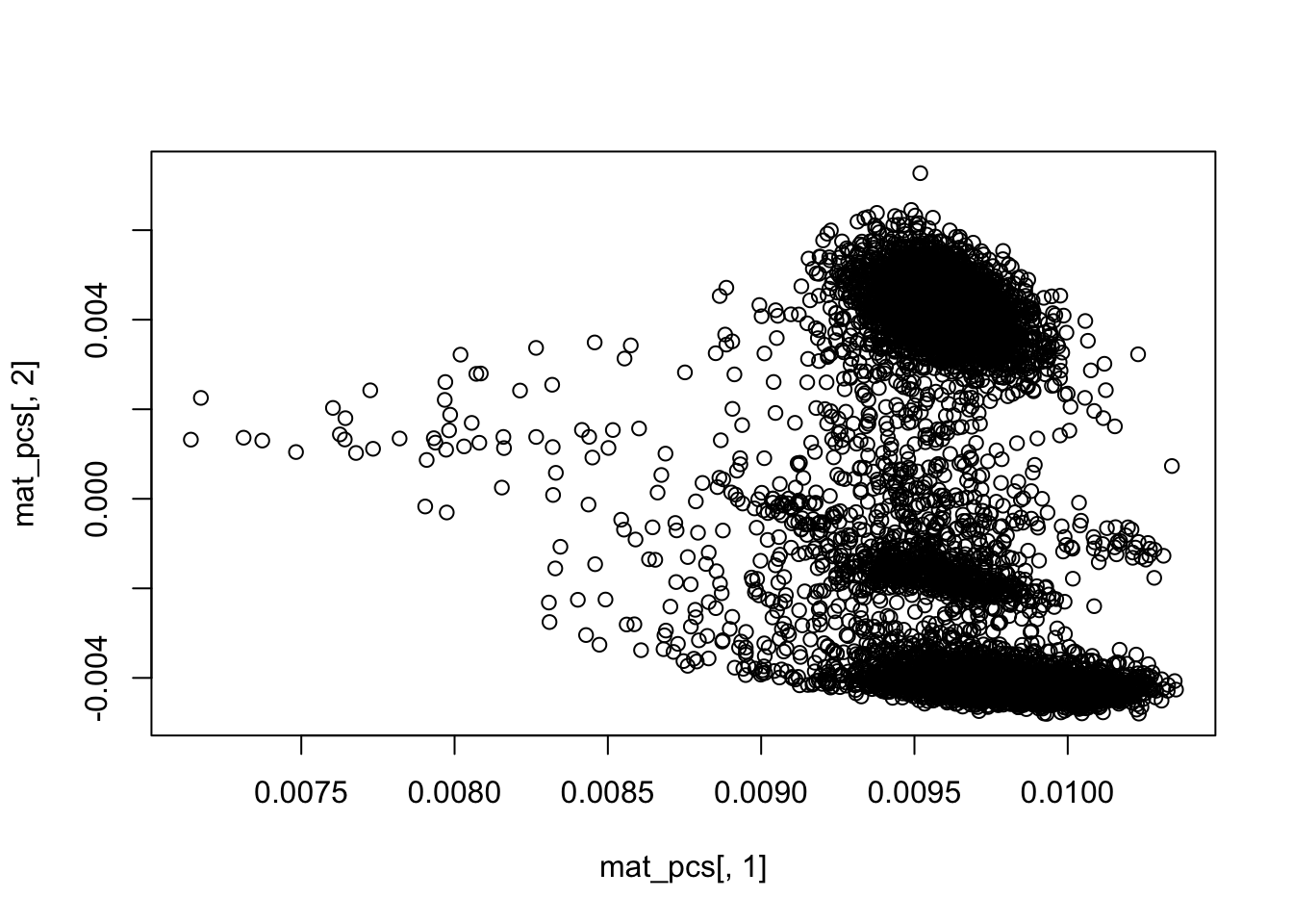

rownames(mat_pcs)<- colnames(mat)

clustering in the PCA space using KNN.

I took some code from Jean Fan’s blog post

library(RANN)
knn.info<- RANN::nn2(mat_pcs, k = 30)

## convert to adjacancy matrix
knn <- knn.info$nn.idx

adj <- matrix(0, nrow(mat_pcs), nrow(mat_pcs))
rownames(adj) <- colnames(adj) <- rownames(mat_pcs)

for(i in seq_len(nrow(mat_pcs))) {
    adj[i,rownames(mat_pcs)[knn[i,]]] <- 1
}

## convert to graph
library(igraph)
g <- igraph::graph.adjacency(adj, mode="undirected")
g <- simplify(g) ## remove self loops

## identify communities, many algorithums. Use the Louvain clustering

km <- igraph::cluster_louvain(g)

com <- km$membership
names(com) <- km$names

# cluster id for each barcode
head(com)

## AAACGAAAGAGCGAAA-1 AAACGAAAGAGTTTGA-1 AAACGAAAGCGAGCTA-1 
##                  7                 14                  2 
## AAACGAAAGGCTTCGC-1 AAACGAAAGTGCTGAG-1 AAACGAACAAGGGTAC-1 
##                 11                  1                 10

## total 13 clusters
table(com)

## com
##    1    2    3    4    5    6    7    8    9   10   11   12   13   14 
## 1776  389  482   34 1100  520  491  640  781  487  204  888  173  763

t-SNE for visualization

library(Rtsne)
library(ggplot2)
library(tibble)
set.seed(345)

mat_tsne<- Rtsne(mat_pcs,  dims = 2, perplexity = 30, verbose = TRUE, 
               max_iter = 1000, check_duplicates = FALSE, is_distance = FALSE, 
               theta = 0.5, pca = FALSE, exaggeration_factor = 12)

## Read the 8728 x 50 data matrix successfully!
## OpenMP is working. 1 threads.
## Using no_dims = 2, perplexity = 30.000000, and theta = 0.500000
## Computing input similarities...
## Building tree...
## Done in 1.81 seconds (sparsity = 0.015574)!
## Learning embedding...
## Iteration 50: error is 94.027001 (50 iterations in 1.63 seconds)
## Iteration 100: error is 80.430931 (50 iterations in 1.34 seconds)
## Iteration 150: error is 77.384844 (50 iterations in 1.10 seconds)
## Iteration 200: error is 76.435871 (50 iterations in 1.12 seconds)
## Iteration 250: error is 75.985857 (50 iterations in 1.16 seconds)
## Iteration 300: error is 2.655848 (50 iterations in 1.02 seconds)
## Iteration 350: error is 2.321504 (50 iterations in 1.02 seconds)
## Iteration 400: error is 2.140627 (50 iterations in 1.05 seconds)
## Iteration 450: error is 2.024543 (50 iterations in 1.06 seconds)
## Iteration 500: error is 1.944114 (50 iterations in 1.06 seconds)
## Iteration 550: error is 1.884803 (50 iterations in 1.10 seconds)
## Iteration 600: error is 1.840703 (50 iterations in 1.14 seconds)
## Iteration 650: error is 1.806387 (50 iterations in 1.06 seconds)
## Iteration 700: error is 1.780991 (50 iterations in 1.07 seconds)
## Iteration 750: error is 1.761708 (50 iterations in 1.07 seconds)
## Iteration 800: error is 1.747014 (50 iterations in 1.10 seconds)
## Iteration 850: error is 1.735953 (50 iterations in 1.07 seconds)
## Iteration 900: error is 1.728716 (50 iterations in 1.11 seconds)
## Iteration 950: error is 1.725798 (50 iterations in 1.13 seconds)
## Iteration 1000: error is 1.724810 (50 iterations in 1.21 seconds)
## Fitting performed in 22.62 seconds.

df_tsne<- as.data.frame(mat_tsne$Y)
colnames(df_tsne)<- c("tSNE1", "tSNE2")
df_tsne$barcode<- rownames(mat_pcs)

df_tsne<- left_join(df_tsne, enframe(com), by = c("barcode" = "name")) %>%
        dplyr::rename(cluster = value) %>%
        mutate(cluster = as.factor(cluster))


ggplot(df_tsne, aes(x = tSNE1, y = tSNE2)) + 
        geom_point(aes(col = cluster), size = 0.5) +
        theme_bw(base_size = 14)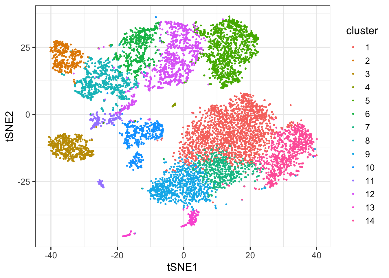

This looks pretty good :)

The easier way: use Seurat

library(Seurat)
peaks <- Read10X_h5(filename = "/Users/mingtang/github_repos/blogdown_data/atac_v1_pbmc_10k_filtered_peak_bc_matrix.h5")

# binarize the matrix
peaks@x[peaks@x >0]<- 1 

## create a seurat object
atac.lsi <- CreateSeuratObject(counts = peaks, assay = 'ATAC', project = '10k_pbmc')

atac.lsi <- RunLSI(object = atac.lsi, n = 50, scale.max = NULL)

# atac.lsi@reductions

atac.lsi<- FindNeighbors(atac.lsi, reduction = "lsi", dims = 1:50)
atac.lsi<- FindClusters(atac.lsi, resolution = 0.8)

## Modularity Optimizer version 1.3.0 by Ludo Waltman and Nees Jan van Eck
## 
## Number of nodes: 8728
## Number of edges: 246454
## 
## Running Louvain algorithm...
## Maximum modularity in 10 random starts: 0.9129
## Number of communities: 20
## Elapsed time: 0 seconds

atac.lsi <- RunTSNE(object = atac.lsi, reduction = "lsi", dims = 1:50)
DimPlot(object = atac.lsi, reduction = 'tsne')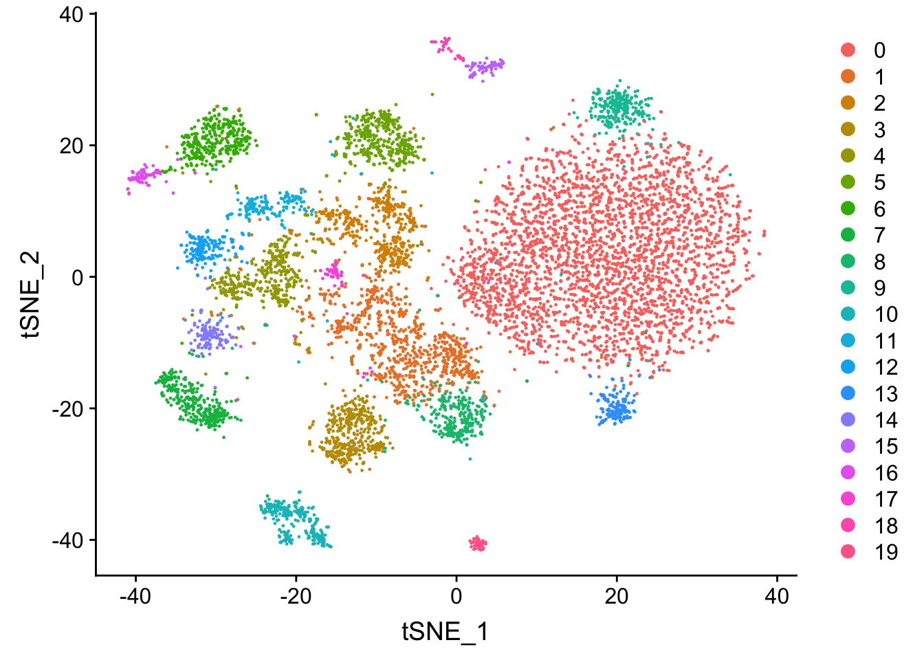

You may argue those two t-SNE graphs look very different in terms of number of clusters and the shape of the clusters. And I agree. There are many reasons for that. I hope Seurat team can give some insights.

The TF-IDF function in Seurat does not do log transformation as in the papers: idf <- log(1+ ncol(x = data) / Matrix::rowSums(x = data))

but rather do a log transformation later: tf.idf <- LogNorm(data = tf.idf, display_progress = verbose, scale_factor = 1e4)

I am not an expert in the graph clustering, but the clustering algorithm in Seurat is probably not exactly the same with igraph::cluster_louvain. Moreover, one can always tweak the k.param and resolution parameters, and the cluster number changes.

We can compare the cell identities for each cluster

# https://github.com/crazyhottommy/scclusteval
library(scclusteval)

# takes two named vector, and calculate the pairwise Jaccard similarity score
# for all clusters
PairWiseJaccardSetsHeatmap(com, Idents(atac.lsi))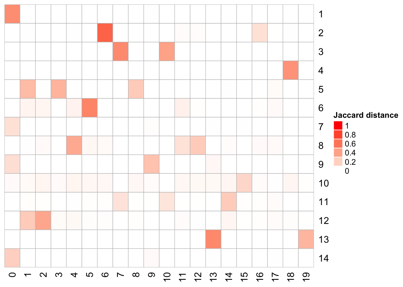

Some other notes

It is known that first dimension is correlated with sequencing depth (although Ansuman et.al did not find such). Nevertheless, if you see such correlation, when cluster cells in the PC space, you can exclude the first PC. e.g. atac.lsi<- FindNeighbors(atac.lsi, reduction = "lsi", dims = 2:50)
I did not do LSI first for crude clustering using the titled 5kb genome bin matrix and call peaks for each crude cluster and then get the count matrix per peak per cell. I am not sure how much this extra work can benefit the clustering.
It turns out the TF-IDF transformation is critical for this sparse matrix. If you do not do it, you will find your t-SNE plot looks really funky! do not trust me, try it yourself:)
for clustering scATAC data, one can use the peak x cell matrix or derive a gene activity score by tools such as Cicero to generate a gene x cell matrix. This is useful when you want to transfer the RNAseq cell type labels to the scATACseq data. see more details in the Seurat V3 paper. The question is then, which matrix should we use for clustering? The clustering of these two different matrix can be different but there should be no surprise. We can use the gene activity score matrix as a label transferring mediator and get the cell labels and then super-impose the cluster id to the t-SNE plot clustered by the peak x cell matrix.

Acknowledgements

I want to thank 10x genomics for making the data publicly available.
I want to thank Jean Fan for putting up some nice posts.
I want to thank Tim Stuart for answering questions with Seurat.
I got some ideas from https://github.com/jaychung10010/Mammary_snATAC-seq as well. Thanks for posting the codes.
I want to thank everyone else who give help and suggestions along my adventure of analyzing scATACseq data.

UPDATE

Do the IF-IDF Seurat way

library(Matrix)
library(readr)
library(dplyr)
mat<- readMM("/Users/mingtang/github_repos/blogdown_data/filtered_peak_bc_matrix/matrix.mtx")
peaks<- read_tsv("/Users/mingtang/github_repos/blogdown_data/filtered_peak_bc_matrix/peaks.bed", col_names = F)
peaks<- peaks %>%
        mutate(id1 = paste(X2, X3, sep = "-")) %>%
        mutate(id = paste(X1, id1, sep = ":"))
        
barcodes<- read_tsv("/Users/mingtang/github_repos/blogdown_data/filtered_peak_bc_matrix/barcodes.tsv", col_names =F)

rownames(mat)<- peaks$id1
colnames(mat)<- barcodes$X1
# binarize the matrix 
mat@x[mat@x >0]<- 1 
# Seurat version TF-IDF
mat<- TF.IDF(mat)
mat<- LogNormalize(mat,scale_factor = 1e4)

### SVD
library(irlba)
set.seed(123)
mat.lsi<- irlba(mat, 50)

d_diagtsne <- matrix(0, 50, 50)
diag(d_diagtsne) <- mat.lsi$d
mat_pcs <- t(d_diagtsne %*% t(mat.lsi$v))
dim(mat_pcs)

## [1] 8728   50

## PCA plot PC1 vs PC2
plot(mat_pcs[,1], mat_pcs[,2])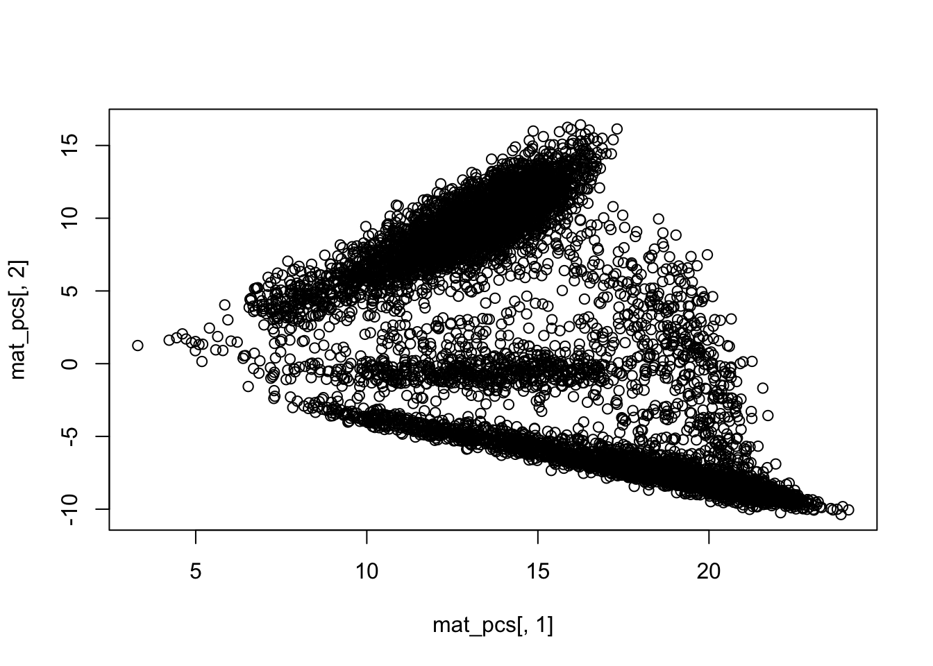

rownames(mat_pcs)<- colnames(mat)

library(RANN)
knn.info<- RANN::nn2(mat_pcs, k = 30)

## convert to adjacancy matrix
knn <- knn.info$nn.idx

adj <- matrix(0, nrow(mat_pcs), nrow(mat_pcs))
rownames(adj) <- colnames(adj) <- rownames(mat_pcs)

for(i in seq_len(nrow(mat_pcs))) {
    adj[i,rownames(mat_pcs)[knn[i,]]] <- 1
}

## convert to graph
library(igraph)
g <- igraph::graph.adjacency(adj, mode="undirected")
g <- simplify(g) ## remove self loops

## identify communities, many algorithums. Use the Louvain clustering

km <- igraph::cluster_louvain(g)

com <- km$membership
names(com) <- km$names

# cluster id for each barcode
head(com)

## AAACGAAAGAGCGAAA-1 AAACGAAAGAGTTTGA-1 AAACGAAAGCGAGCTA-1 
##                 13                  7                 12 
## AAACGAAAGGCTTCGC-1 AAACGAAAGTGCTGAG-1 AAACGAACAAGGGTAC-1 
##                 14                 13                 16

## total 13 clusters
table(com)

## com
##    1    2    3    4    5    6    7    8    9   10   11   12   13   14   15 
##  801  376  617  629  572   56  607  435  280  390  131  417 2554  490  241 
##   16 
##  132

### T-sne visualization
library(Rtsne)
library(ggplot2)
library(tibble)
set.seed(345)

mat_tsne<- Rtsne(mat_pcs,  dims = 2, perplexity = 30, verbose = TRUE, 
               max_iter = 1000, check_duplicates = FALSE, is_distance = FALSE, 
               theta = 0.5, pca = FALSE, exaggeration_factor = 12)

## Read the 8728 x 50 data matrix successfully!
## OpenMP is working. 1 threads.
## Using no_dims = 2, perplexity = 30.000000, and theta = 0.500000
## Computing input similarities...
## Building tree...
## Done in 2.57 seconds (sparsity = 0.014984)!
## Learning embedding...
## Iteration 50: error is 94.871477 (50 iterations in 1.48 seconds)
## Iteration 100: error is 84.409610 (50 iterations in 1.50 seconds)
## Iteration 150: error is 82.319098 (50 iterations in 1.18 seconds)
## Iteration 200: error is 81.831573 (50 iterations in 1.35 seconds)
## Iteration 250: error is 81.608255 (50 iterations in 1.40 seconds)
## Iteration 300: error is 3.039995 (50 iterations in 1.20 seconds)
## Iteration 350: error is 2.691975 (50 iterations in 1.14 seconds)
## Iteration 400: error is 2.508723 (50 iterations in 1.24 seconds)
## Iteration 450: error is 2.390684 (50 iterations in 1.14 seconds)
## Iteration 500: error is 2.308249 (50 iterations in 1.16 seconds)
## Iteration 550: error is 2.248218 (50 iterations in 1.12 seconds)
## Iteration 600: error is 2.201765 (50 iterations in 1.27 seconds)
## Iteration 650: error is 2.166028 (50 iterations in 1.21 seconds)
## Iteration 700: error is 2.137659 (50 iterations in 1.13 seconds)
## Iteration 750: error is 2.115987 (50 iterations in 1.11 seconds)
## Iteration 800: error is 2.098913 (50 iterations in 1.16 seconds)
## Iteration 850: error is 2.086752 (50 iterations in 1.08 seconds)
## Iteration 900: error is 2.079435 (50 iterations in 1.07 seconds)
## Iteration 950: error is 2.078012 (50 iterations in 1.14 seconds)
## Iteration 1000: error is 2.076638 (50 iterations in 1.12 seconds)
## Fitting performed in 24.21 seconds.

df_tsne<- as.data.frame(mat_tsne$Y)
colnames(df_tsne)<- c("tSNE1", "tSNE2")
df_tsne$barcode<- rownames(mat_pcs)

df_tsne<- left_join(df_tsne, enframe(com), by = c("barcode" = "name")) %>%
        dplyr::rename(cluster = value) %>%
        mutate(cluster = as.factor(cluster))

ggplot(df_tsne, aes(x = tSNE1, y = tSNE2)) + 
        geom_point(aes(col = cluster), size = 0.5) +
        theme_bw(base_size = 14)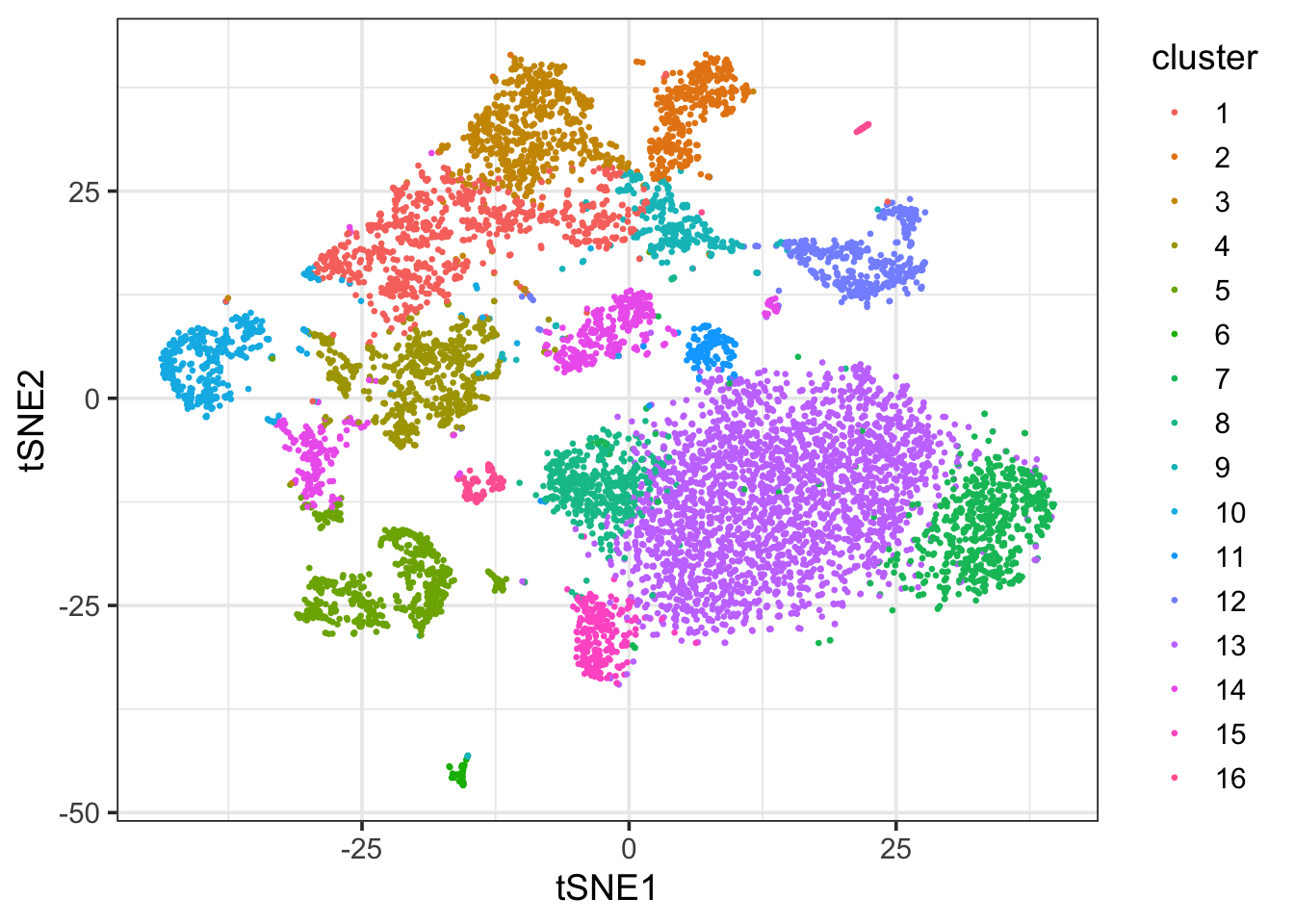

Well, it still looks different from the Seurat output. Any comments?

ATACseq single-cell R