I asked this question on Twitter:
what test to test if two distributions are different? I am aware of KS test. When n is large (which is common in genomic studies), the p-value is always significant. better to test against an effect size? how to do it in this context?
In genomics studies, it is very common to have large N (e.g., the number of introns, promoters in the genome, number of cells in the single-cell studies). A more concrete example is that one have two samples: control and treatment. one can calculate the intron retention level for each intron across the genome and ask if globally the distribution of the intron retention scores is different between the control sample and treatment sample.
Kolmogorov–Smirnov test
I am aware of the Kolmogorov–Smirnov test (K–S test or KS test).
The Kolmogorov–Smirnov statistic quantifies a distance between the empirical distribution function of the sample and the cumulative distribution function of the reference distribution, or between the empirical distribution functions of two samples.
Kolmogorov–Smirnov statistic is used in the popular GSEA too. It is good to see some examples.
We will use random sampling from normal distribution as examples.
library(tidyverse)
library(patchwork)

test_distribution<- function(N, mean1, mean2, sd1, sd2){
  set.seed(123)
  ## random sample from normal distribution
  x<- rnorm(N, mean=mean1, sd = sd1)
  set.seed(234)
  y<- rnorm(N, mean=mean2, sd = sd2)

  df<- data.frame(x=x, y =y)

  ## make it long format
  df<- df %>%
    pivot_longer(cols = 1:2, names_to = "group", values_to = "value")
  ## check the ECDF for the two distributions
  p1<- ggplot(df, aes(value)) +
    stat_ecdf(geom = "step", aes(color = group)) +
    theme_classic(base_size = 14) +
    ylab("Cumulative probability") +
    ggtitle("ECDF for x and y", subtitle = glue::glue( "x ~ N({mean1}, {sd1})\n y ~ N({mean2}, {sd2})"))


  p2<- ggplot(df, aes(x= group, y = value)) +
    geom_boxplot(aes(fill = group)) +
    theme_classic(base_size = 14) +
    ggtitle(paste0("N = ", N))

  p<- p1 + p2

  ks<- ks.test(x,y)
  t<- t.test(x,y)
  return(list(ks = ks, ttest =t, p = p, df = df))

}


res<- test_distribution(1000, 0, 0, 1, 1)
res$p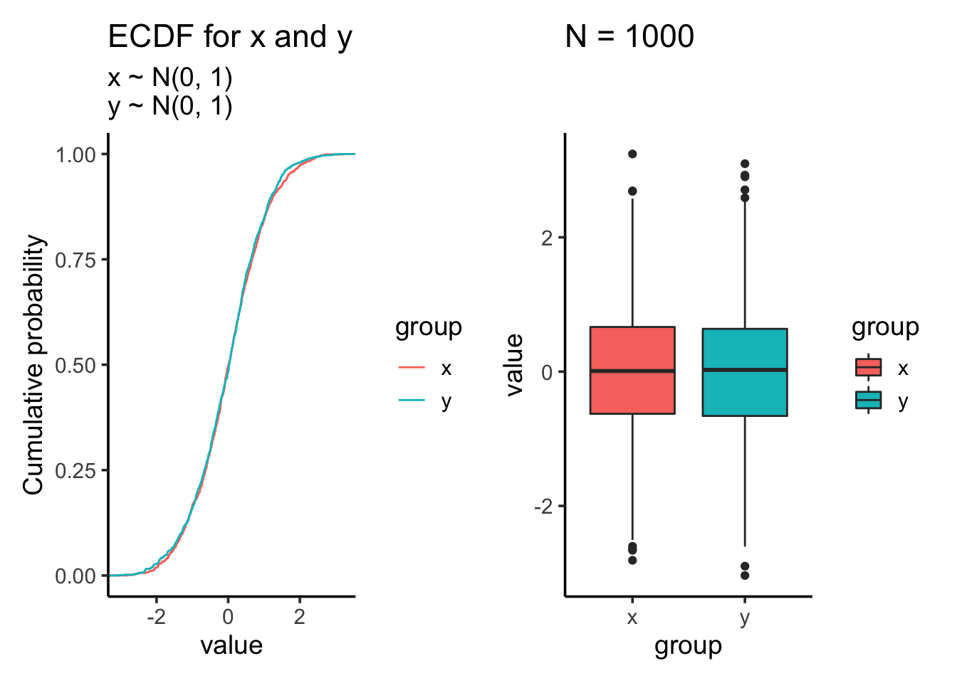
res$ks##
## Two-sample Kolmogorov-Smirnov test
##
## data: x and y
## D = 0.025, p-value = 0.9135
## alternative hypothesis: two-sidedKS test showing the distribution is not significantly different which makes sense as we draw samples from the same normal distribution.
res$ttest##
## Welch Two Sample t-test
##
## data: x and y
## t = 0.85389, df = 1997.9, p-value = 0.3933
## alternative hypothesis: true difference in means is not equal to 0
## 95 percent confidence interval:
## -0.04893966 0.12442136
## sample estimates:
## mean of x mean of y
## 0.01612787 -0.02161298Two sample t test shows that the mean is not significantly different.
Let’s increase the standard deviation for the second sample to 1.2
res<- test_distribution(1000, 0, 0, 1, 1.2)
res$p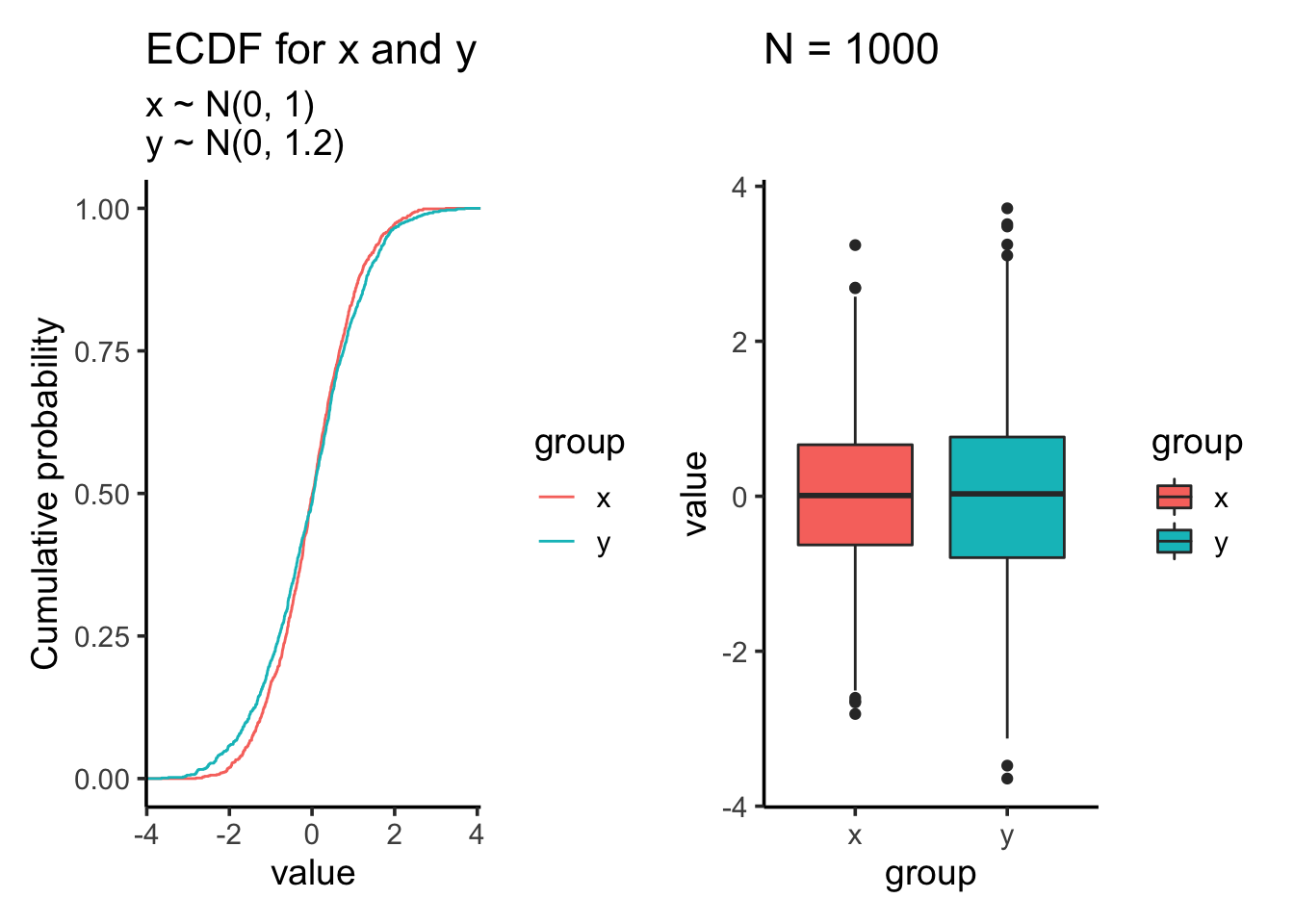
res$ks##
## Two-sample Kolmogorov-Smirnov test
##
## data: x and y
## D = 0.053, p-value = 0.1205
## alternative hypothesis: two-sidedres$ttest##
## Welch Two Sample t-test
##
## data: x and y
## t = 0.86215, df = 1939.5, p-value = 0.3887
## alternative hypothesis: true difference in means is not equal to 0
## 95 percent confidence interval:
## -0.05362088 0.13774778
## sample estimates:
## mean of x mean of y
## 0.01612787 -0.02593558Let’s increase the sample size
res<- test_distribution(10000, 0, 0, 1, 1.2)
res$p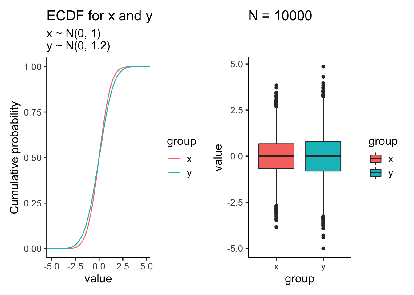
res$ks##
## Two-sample Kolmogorov-Smirnov test
##
## data: x and y
## D = 0.0497, p-value = 3.746e-11
## alternative hypothesis: two-sidedres$ttest##
## Welch Two Sample t-test
##
## data: x and y
## t = 0.19585, df = 19342, p-value = 0.8447
## alternative hypothesis: true difference in means is not equal to 0
## 95 percent confidence interval:
## -0.02758649 0.03371124
## sample estimates:
## mean of x mean of y
## -0.002371702 -0.005434073After we increase the sample size, t-test which tests against mean is still not significant. However, the KS test becomes highly significant even the samples are drew from the same two distributions as the last comparison!!
Let’s try another example with very small difference (small here is subjective, one has to decide it under the experiment context) of means.
res<- test_distribution(1000, 0, 0.1, 1, 1)
res$p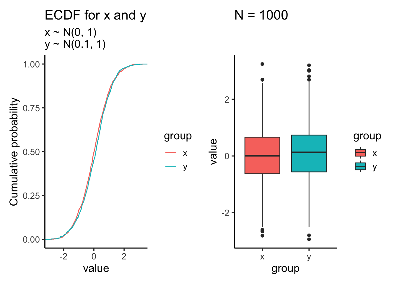
res$ks##
## Two-sample Kolmogorov-Smirnov test
##
## data: x and y
## D = 0.054, p-value = 0.1083
## alternative hypothesis: two-sidedres$ttest##
## Welch Two Sample t-test
##
## data: x and y
## t = -1.4086, df = 1997.9, p-value = 0.1591
## alternative hypothesis: true difference in means is not equal to 0
## 95 percent confidence interval:
## -0.14893966 0.02442136
## sample estimates:
## mean of x mean of y
## 0.01612787 0.07838702Let’s increase the sample size to 10000:
res<- test_distribution(10000, 0, 0.1, 1, 1)
res$p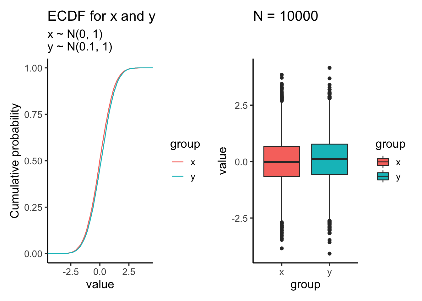
res$ks##
## Two-sample Kolmogorov-Smirnov test
##
## data: x and y
## D = 0.0502, p-value = 2.273e-11
## alternative hypothesis: two-sidedres$ttest##
## Welch Two Sample t-test
##
## data: x and y
## t = -6.914, df = 19998, p-value = 4.853e-12
## alternative hypothesis: true difference in means is not equal to 0
## 95 percent confidence interval:
## -0.12558133 -0.07010528
## sample estimates:
## mean of x mean of y
## -0.002371702 0.095471606Suddenly, both the KS test and t-test becomes highly significant after increasing the sample size.
That’s why we should not put too much emphasis on the p-values, but also check the effect size. Many genomic papers show highly significant p values < 2.22e−16 (smallest you can get from R) simply because the sample size is really big (I have to confess that I have it too in my papers because my PI/reviewers asked).
earth mover distance (EMD)
Others in the tweet thread mentioned earth mover distance that can be used to measure the distance between two distributions. There is a biconductor package for calculating it. The EMDomics algorithm is used to perform a supervised multi-class analysis to measure the magnitude and statistical significance of observed continuous genomics data between groups.
library(EMDomics)


calculate_EMD<- function(df){
  num<- 1:nrow(df)
  exp_data<- df$value
  names(exp_data)<- glue::glue("sample_{num}")
  labels<- df$group
  names(labels)<- names(exp_data)
  calculate_emd_gene(exp_data, labels, names(exp_data))
}

res<- test_distribution(1000, 0, 0, 1, 1.2)
calculate_EMD(res$df)
## [1] 0.7629998## increase the sample size
res<- test_distribution(10000, 0, 0, 1, 1.2)
calculate_EMD(res$df)## [1] 0.8505res<- test_distribution(1000, 0, 0.1, 1, 1)
calculate_EMD(res$df)## [1] 0.3919999res$df %>% head()## # A tibble: 6 x 2
## group value
## <chr> <dbl>
## 1 x -0.560
## 2 y 0.761
## 3 x -0.230
## 4 y -1.95
## 5 x 1.56
## 6 y -1.40res<- test_distribution(10000, 0, 0.1, 1, 1)
calculate_EMD(res$df)## [1] 0.4892001Two observations:
- EMD between \(N(0,1)\) and \(N(0.1,1)\) is smaller than EMD between \(N(0,1)\) and \(N(0,1.2)\)
- increasing the sample size will increase the EMD too!
The EMD score increases as the distributions become increasingly dissimilar, but we have no framework for estimating the significance of a particular EMD score. EMDomics uses a permutation-based method to calculate a q-value that is interpreted analogously to a p-value.
The EMDomics packages implemented the permutation test for multiple genes. Let me do it for a single gene.
res<- test_distribution(1000, 0, 0, 1, 1.2)
res$df
## # A tibble: 2,000 x 2
## group value
## <chr> <dbl>
## 1 x -0.560
## 2 y 0.793
## 3 x -0.230
## 4 y -2.46
## 5 x 1.56
## 6 y -1.80
## 7 x 0.0705
## 8 y 1.77
## 9 x 0.129
## 10 y 1.75
## # … with 1,990 more rowscalculate_EMD(res$df)## [1] 0.7629998## random shuffle the x, y group designation and calculate the EMD score
permutation_EMD<- function(d){
set.seed(NULL)
d$group<- sample(d$group)
calculate_EMD(d)
}
permutation_EMD(res$df)## [1] 0.165## a different shuffle gives a different EMD
permutation_EMD(res$df)## [1] 0.511## permutate N times and calculate how many times the permutated EMD is bigger than the EMD
## for the original data and that's the p-value
permutation_EMD_pvalue<- function(d, N_permutation = 1000){
permutation_EMDs<- replicate(N_permutation, permutation_EMD(d))
### p-value
mean(calculate_EMD(d) < permutation_EMDs)
}
permutation_EMD_pvalue(res$df)## [1] 0.003The p-value is < 0.05 which suggests that the two distributions are significantly different.
If we sample from the same \(N(0,1)\) distribution:
res<- test_distribution(1000, 0, 0, 1, 1)
permutation_EMD_pvalue(res$df)
## [1] 0.602p-value is not significant.
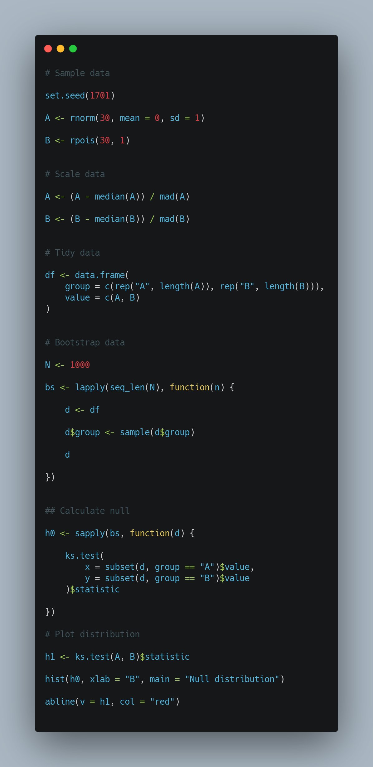
In fact, many people suggested using a permutation based method to evaluate the significance of the distribution differences using the KS test. The below code snippet is from James:
Comparing groups of distributions
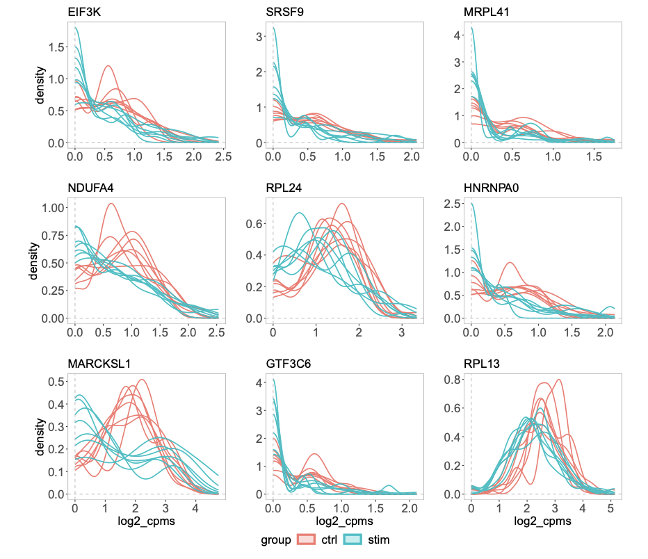
For scRNAseq or CyTOF data, if one has treatment vs control groups, 3 samples each, each sample contains 1000 cells. How to test if the treatment changes the expression of a certain gene? This is an example of multi-sample, multi-group single-cell differential analysis. Pseudo-bulk method can be used as in the muscat. Note that it is different from marker gene identification where differential gene expression is carried out between clusters of cells.
Papers to read:
quantro: a data-driven approach to guide the choice of an appropriate normalization method
Fast identification of differential distributions in single-cell RNA-sequencing data with waddR
distinct: a novel approach to differential distribution analyses
Rafa, our department chair asked a good question:
First I would ask why is testing for a difference in mean and a difference in SD not enough? Can you construct examples of two distributions with the same mean and same SD but different in a meaningful way in your context? Seeing these examples will help motivate a solution.
— Rafael Irizarry (@rafalab) July 14, 2021
Figure 7 b from the distinct paper shows some genes have different distributions but have the same mean across groups.